4.6 Graph Sketching and Asymptotes
In this section, our goal is to sketch graphs using the information provided by the first two derivatives \(f'\) and \(f''\). We will see that a useful sketch can be produced without plotting a large number of points. Although nowadays almost all graphs are produced by computer (including, of course, the graphs in this textbook), sketching graphs by hand is a useful way of solidifying your understanding of the basic concepts in this chapter.
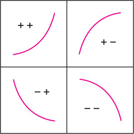
Most graphs are made up of smaller arcs that have one of the four basic shapes, corresponding to the four possible sign combinations of \(f'\) and \(f''\) (Figure 4.52). Since \(f'\) and \(f''\) can each have sign \(+\) or \(-\), the sign combinations are
\[ ++\qquad+-\qquad-+\qquad-- \]
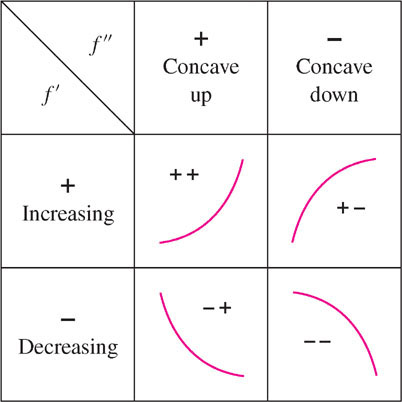
In this notation, the first sign refers to \(f'\) and the second sign to \(f''\). For instance, \(-+\) indicates that \(f'(x) < 0\) and \(f''(x) > 0\).
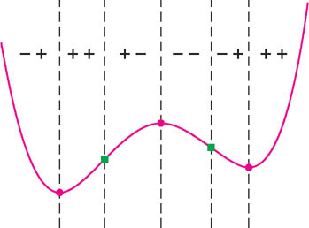
In graph sketching, we focus on the transition points, where the basic shape changes due to a sign change in either \(f'\) (local min or max) or \(f''\) (point of inflection). In this section, local extrema are indicated by solid dots, and points of inflection are indicated by green solid squares (Figure 4.53).
In graph sketching, we must also pay attention to asymptotic behavior—that is, to the behavior of \(f(x)\) as \(x\) approaches either \(\pm \infty\) or a vertical asymptote.
The next three examples treat polynomials. Recall from Section 2.7 that the limits at infinity of a polynomial
\[ f(x) = a_nx^n + a_{n-1}x^{n-1}+\cdots+a_1x+a_0 \]
249
(assuming that \(a_{n} \neq 0\)) are determined by
\[ \lim\limits_{x\rightarrow \pm\infty}f(x) = a_n\lim\limits_{x\rightarrow \pm\infty} \]
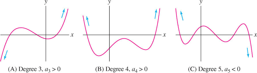
In general, then, the graph of a polynomial “wiggles” up and down a finite number of times and then tends to positive or negative infinity (Figure 4.54).
Example 1 Quadratic Polynomial
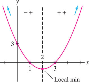
Sketch the graph of \(f(x) = x^{2} - 4x + 3\).
Solution We have \(f'(x) = 2x - 4 = 2(x - 2)\). We can see directly that \(f'(x)\) is negative for \(x < 2\) and positive for \(x > 2\), but let’s confirm this using test values, as in previous sections:
| Interval | Test Value | Sign of \(f'\) |
|---|---|---|
| \((-\infty , 2)\) | \(f'(1) = -2\) | \(-\) |
| \((2,\infty )\) | \(f'(3) = 2\) | \(+\) |
Furthermore, \(f''(x) = 2\) is positive, so the graph is everywhere concave up. To sketch the graph, plot the local minimum \((2, -1)\), the \(y\)-intercept, and the roots \(x = 1, 3\). Since the leading term of \(f\) is \(x^{2}\), \(f(x)\) tends to \(\infty\) as \(x \rightarrow \pm \infty\) . This asymptotic behavior is noted by the arrows in Figure 4.55.
Example 2 Cubic Polynomial
Sketch the graph of \(f(x)=\frac{1}{3}x^3 -\frac{1}{2}x^2 - 2x + 3\).
Solution
Step 1. Determine the signs of \(f'\) and \(f''\).
First, solve for the critical points:
\[ f'(x) = x^{2} - x - 2 = (x + 1)(x - 2) = 0 \]
The critical points \(c = -1, 2\) divide the \(x\)-axis into three intervals \((-\infty , -1)\), \((-1, 2)\), and \((2, \infty )\), on which we determine the sign of \(f'\) by computing test values:
| Interval | Test Value | Sign of \(f'\) |
|---|---|---|
| \((-\infty , -1)\) | \(f'(-2) = 4\) | \(+\) |
| \((-1, 2)\) | \(f'(0) = -2\) | \(-\) |
| \((2, \infty )\) | \(f'(3) = 4\) | \(+\) |
Next, solve \(f''(x) = 2x - 1 = 0\). The solution is \(c=\frac{1}{2}\) and we have
| Interval | Test Value | Sign of \(f''\) |
|---|---|---|
| \(\left(-\infty,\frac{1}{2}\right)\) | \(f''(0) = -1\) | \(-\) |
| \(\left(\frac{1}{2},\infty\right)\) | \(f''(1) = 1\) | \(+\) |
250
Step 2. Note transition points and sign combinations.
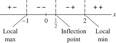
This step merges the information about \(f'\) and \(f''\) in a sign diagram (Figure 4.56). There are three transition points:
- \(c = -1\): local max since \(f'\) changes from \(+\) to \(-\) at \(c = -1\).
- \(c=\frac{1}{2}\): point of inflection since \(f''\) changes sign at \(c=\frac{1}{2}\).
- \(c = 2\): local min since \(f'\) changes from \(-\) to \(+\) at \(c = 2\).
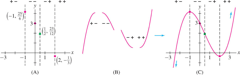
In Figure 4.57(A), we plot the transition points and, for added accuracy, the \(y\)-intercept \(f(0)\), using the values
\[ f(-1) = \frac{25}{6},\qquad f\left(\frac{1}{2}\right)= \frac{23}{12},\qquad f(0)=3,\qquad f(2) = -\frac{1}{3} \]
Step 3. Draw arcs of appropriate shape and asymptotic behavior.
The leading term of \(f(x)\) is \(\frac{1}{3}x^3\). Therefore, \(\lim\limits_{x\rightarrow \infty}f(x)=\infty\) and \(\lim\limits_{x\rightarrow -\infty}f(x)=-\infty\).
To create the sketch, it remains only to connect the transition points by arcs of the appropriate concavity and asymptotic behavior, as in Figure 4.57(B) and (C).
Example 3
Sketch the graph of \(f(x) = 3x^{4} - 8x^{3} + 6x^{2} + 1\).
Solution
Step 1. Determine the signs of \(f'\) and \(f''\).
First, solve for the transition points:
\begin{align*} f'(x) = 12x^3 - 24x^2 + 12x = 12x(x-1)^2 &=0\implies x=0,1\\ f''(x) = 36x^2 - 48x + 12 = 12(x-1)(3x-1)&=0\implies x=\frac{1}{3},1 \end{align*}
The signs of \(f'\) and \(f''\) are recorded in the following tables.
| Interval | Test Value | Sign of \(f'\) |
|---|---|---|
| \((-\infty , 0)\vphantom{\left(-\infty,\frac{1}{3}\right)}\) | \(f'(-1) = -48\) | \(-\) |
| \((0, 1)\) | \(f\left(\frac{1}{2}\right)=\frac{3}{2}\) | \(+\) |
| \((1, \infty )\) | \(f'(2) = 24\) | \(+\) |
| Interval | Test Value | Sign of \(f''\) |
|---|---|---|
| \(\left(-\infty,\frac{1}{3}\right)\) | \(f''(0) = 12\) | \(+\) |
| \(\left(\frac{1}{3},1\right)\) | \(f\left(\frac{1}{2}\right) = -3\) | \(-\) |
| \((1, \infty )\) | \(f''(2) = 60\) | \(+\) |
Step 2. Note transition points and sign combinations.
The transition points \(c=0,\frac{1}{3},1\) divide the \(x\)-axis into four intervals (Figure 4.58). The type of sign change determines the nature of the transition point:
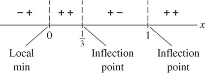
- \(c = 0\): local min since \(f'\) changes from \(-\) to \(+\) at \(c = 0\).
- \(c=\frac{1}{3}\): point of inflection since \(f''\) changes sign at \(c=\frac{1}{3}\).
251
- \(c = 1\): neither a local min nor a local max since \(f'\) does not change sign, but it is a point of inflection since \(f''(x)\) changes sign at \(c = 1\).
We plot the transition points \(c=0,\frac{1}{3}, 1\) in Figure 4.59(A) using function values \(f(0) = 1\), \(f\left(\frac{1}{3}\right)=\frac{38}{27}\), and \(f(1) = 2\).
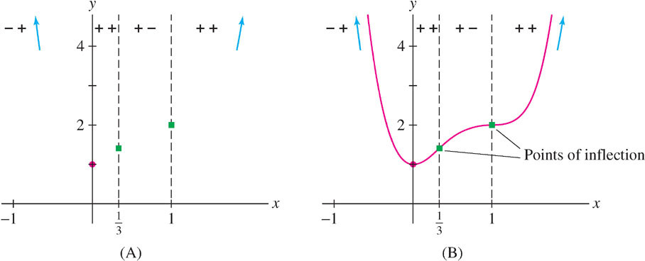
Step 3. Draw arcs of appropriate shape and asymptotic behavior.
Before drawing the arcs, we note that \(f(x)\) has leading term \(3x^{4}\), so \(f(x)\) tends to \(\infty\) as \(x \rightarrow \infty\) and as \(x \rightarrow -\infty\). We obtain Figure 4.59(B).
Example 4 Trigonometric Function
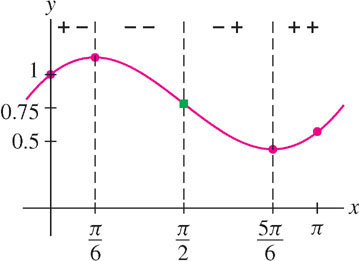
Sketch \(f(x)=\cos x+\frac{1}{2}x\) over \([0, \pi ]\).
Solution First, we solve the transition points for \(x \in [0, \pi ]\):
\begin{eqnarray*} f'(x)&=&-\sin x + \frac{1}{2}=0 &\implies&x=\frac{\pi}{6},\frac{5\pi}{6}\\ f''(x)&=&-\cos x=0&\implies&x=\frac{\pi}{2} \end{eqnarray*}
The sign combinations are shown in the following tables.
| Interval | Test Value | Sign of \(f'\) |
|---|---|---|
| \(\left(0,\frac{\pi}{6}\right)\) | \(f'\left(\frac{\pi}{12}\right)\approx0.24\) | \(+\) |
| \(\left(\frac{\pi}{6},\frac{5\pi}{6}\right)\) | \(f'\left(\frac{\pi}{2}\right) = -\frac{1}{2}\) | \(-\) |
| \(\left(\frac{5\pi}{6},\pi\right)\) | \(f'\left(\frac{11\pi}{12}\right)\) | \(+\) |
| Interval | Test Value | Sign of \(f''\) |
|---|---|---|
| \(\left(0,\frac{\pi}{2}\right)\) | \(f''\left(\frac{\pi}{4}\right) = -\frac{\sqrt{2}}{2}\) | \(-\) |
| \(\left(\frac{\pi}{2},\pi\right)\) | \(f''\left(\frac{3\pi}{4}\right) = \frac{\sqrt{2}}{2}\) | \(+\) |
We record the sign changes and transition points in Figure 4.60 and sketch the graph using the values
\[ f(0) = 1,\quad f\left(\frac{\pi}{6}\right)\approx1.13,\quad f\left(\frac{5\pi}{6}\right)\approx0.44,\quad f(\pi) \approx 0.57 \]
Example 5 A Function Involving \(e^{x}\)
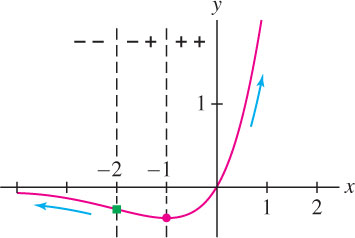
Sketch the graph of \(f(x) = xe^{x}\).
Solution As usual, we solve for the transition points and determine the signs:
\begin{align*} f'(x)=xe^x+ e^x = (x+1)e^x&=0\implies x=-1\\ f''(x)=(x+1)e^x + e^x (x+2)e^x&=0\implies x=-2 \end{align*}
252
| Interval Test | Value | Sign of \(f'\) |
|---|---|---|
| \((-\infty ,-1)\) | \(f'(-2) = -e^{-2}\) | \(-\) |
| \((-1,\infty )\) | \(f'(0) = e^{0}\) | \(+\) |
| Interval Test | Value | Sign of \(f''\) |
|---|---|---|
| \((-\infty ,-2)\) | \(f''(-3) = -e^{-3}\) | \(-\) |
| \((-2,\infty )\) | \(f'' (0) = 2e^{0}\) | \(+\) |
The sign change of \(f'\) shows that \(f(-1)\) is a local min. The sign change of \(f''\) shows that \(f\) has a point of inflection at \(x = -2\), where the graph changes from concave down to concave up.
The last pieces of information we need are the limits at infinity. Both \(x\) and \(e^{x}\) tend to \(\infty\) as \(x \rightarrow \infty\) , so \(\lim\limits_{x\rightarrow \infty}xe^x=\infty\). On the other hand, the limit as \(x \rightarrow -\infty\) is indeterminate of type \(\infty \cdot 0\) because \(x\) tends to \(-\infty\) and \(e^{x}\) tends to zero. Therefore, we write \(xe^{x} = \frac{x}{e^{-x}}\) and apply L’Hôpital’s Rule:
\[ \lim\limits_{x\rightarrow -\infty}xe^x= \lim\limits_{x\rightarrow -\infty}\frac{x}{e^{-x}}= \lim\limits_{x\rightarrow -\infty}\frac{1}{-e^{-x}}= -\lim\limits_{x\rightarrow -\infty}{e^{x}}=0 \]
Figure 4.61 shows the graph with its local minimum and point of inflection, drawn with the correct concavity and asymptotic behavior.
The next two examples deal with horizontal and vertical asymptotes.
Example 6
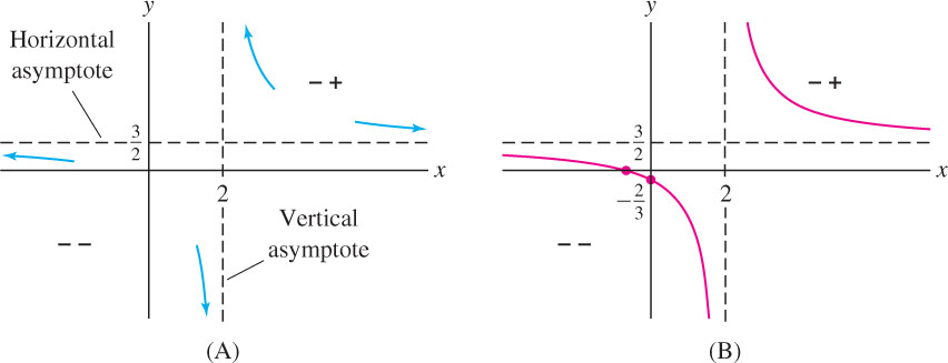
Sketch the graph of \(f(x) = \dfrac{3x+2}{2x-4}\).
Solution The function \(f(x)\) is not defined for all \(x\). This plays a role in our analysis so we add a Step 0 to our procedure.
Step 0. Determine the domain of \(f\).
Since \(f(x)\) is not defined for \(x = 2\), the domain of \(f\) consists of the two intervals \((-\infty , 2)\) and \((2, \infty )\). We must analyze \(f\) on these intervals separately.
Step 1. Determine the signs of \(f'\) and \(f''\).
Calculation shows that
\[ f'(x)=-\frac{4}{(x-2)^2}\qquad f''(x)=\frac{8}{(x-2)^3} \]
Although \(f'(x)\) is not defined at \(x = 2\), we do not call it a critical point because \(x = 2\) is not in the domain of \(f\). In fact, \(f'(x)\) is negative for \(x \neq 2\), so \(f(x)\) is decreasing and has no critical points.
On the other hand, \(f''(x) > 0\) for \(x > 2\) and \(f''(x) < 0\) for \(x < 2\). Although \(f''(x)\) changes sign at \(x = 2\), we do not call \(x = 2\) a point of inflection because it is not in the domain of \(f\).
Step 2. Note transition points and sign combinations.
There are no transition points in the domain of f.
| \((-\infty , 2)\) | \(f'(x) < 0\) and \(f''(x) < 0\) |
| \((2, \infty )\) | \(f'(x) < 0\) and \(f''(x) > 0\) |
Step 3. Draw arcs of appropriate shape and asymptotic behavior.
The following limits show that \(y=\frac{3}{2}\) is a horizontal asymptote:
\[ \lim\limits_{x\rightarrow \pm\infty} \frac{3x+2}{2x-4}= \lim\limits_{x\rightarrow \pm\infty} \frac{3+2x^{-1}}{2-4x^{-1}}= \frac{3}{2} \]
253
The line \(x = 2\) is a vertical asymptote because \(f(x)\) has infinite one-sided limits
\[ \lim\limits_{x\rightarrow 2^-}\frac{3x+2}{2x-4}=-\infty\quad \lim\limits_{x\rightarrow 2^+}\frac{3x+2}{2x-4}=\infty \]
To verify this, note that for \(x\) near 2, the denominator \(2x - 4\) is small negative if \(x < 2\) and small positive if \(x > 2\), whereas the numerator \(3x + 4\) is positive.
Example 7
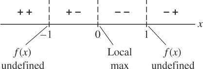
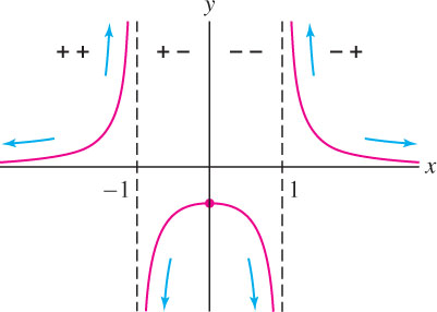
Sketch the graph of \(f(x)=\dfrac{1}{x^2-1}\).
Solution The function \(f(x)\) is defined for \(x \neq \pm 1\). By calculation,
\[ f'(x)=-\frac{2x}{(x^2-1)^2}\qquad f''(x)=\frac{6x^2+2}{(x^2-1)^3} \]
For \(x \neq \pm 1\), the denominator of \(f'(x)\) is positive. Therefore, \(f'(x)\) and \(x\) have opposite signs:
- \(f'(x) > 0\) for \(x < 0\), \(f'(x) < 0\) for \(x > 0\), \(x = 0\) is a local max.
The sign of \(f''(x)\) is equal to the sign of \(x^{2} - 1\) because \(6x^{2} + 2\) is positive:
- \(f''(x) > 0\) for \(x < -1\) or \(x > 1\) and \(f''(x) < 0\) for \(-1 < x < 1\).
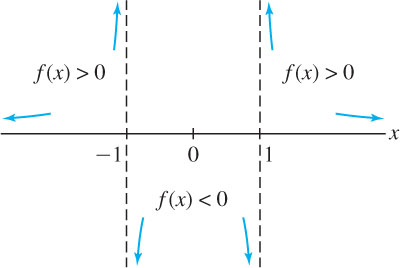
Figure 4.63 summarizes the sign information.
The \(x\)-axis, \(y = 0\), is a horizontal asymptote because
\[ \lim\limits_{x\rightarrow \infty}\frac{1}{x^2-1}=0 \quad\text{and}\quad \lim\limits_{x\rightarrow -\infty}\frac{1}{x^2-1}=0 \]
In this example,
\begin{align*} f(x)&=\frac{1}{x^2-1}\\ f'(x)&=-\frac{2x}{(x^2-1)^2}\\ f''(x)&=\frac{6x^2+2}{(x^2-1)^3}\\ \end{align*}
| Vertical Asymptote | Left-Hand Limit | Right-Hand Limit |
|---|---|---|
| \(x = -1\) | \(\lim\limits_{x\rightarrow -1^-}\dfrac{1}{x^2-1}=\infty\) | \(\lim\limits_{x\rightarrow -1^+}\dfrac{1}{x^2-1}=-\infty\) |
| \(x = 1\) | \(\lim\limits_{x\rightarrow 1^-}\dfrac{1}{x^2-1}=-\infty\) | \(\lim\limits_{x\rightarrow 1^+}\dfrac{1}{x^2-1}=\infty\) |
Question 4.21 Graph Sketching and Asymptotes Progress Check Question 1
sDfXYwLDs0VhuGvoWUjhMyXbuwovmD/Ymrbb4LbSJ7Rhl7ykNv5PtQ5l9xznCG2knwADP8kpoSYc2WxaN8nIVtChAmrqqy/68a2uAMGY12QJUUQEw+SuFHSd8xdJ+/Qs7SyTFr0JMs/ElEk8+fW7/UzanyFZGyqBccTlTETkFLNwKHcJ4WgIQglTPYKbTdnsw0kZPlNEYaIrbak32H1c89DAScPcIvKyd7UAdxYdz1xoZnfb49Io+5WzPcFqMfvIF3yRzmvE15LlMFqHVWTsQLahSFsTr32atZbrpUZM5VoXDWZBC53qNr2a0dRgdtlMx33qeYeGJ3t/uK7jx1sAhuhRat40oq7DdoEFYTu2D+iTi/Qsk0h60Ey7EIUxKAkZtrPEp1ozZ8zrIlQEgPFA6Y/DN2wS5eyQeBFAFBoglOweEQVbd1pNi8lgZG/Pc4riQee+lxQ4/dtTYJDZeVhSkG0FRHYPmzvYC79Oy2JrpaVQRzMhSJcdVPeLwRcZGPZ2NWbyKZ2wqoL0sBCBTU8KBjAKYKaceA7ncmhw8Kh4/5aXhuu/MkYq0T8SWDoJTKb8UnmPrUZxyfXMrCmC49oKPmVv2ZXvVZEwhAqiNfZBpXbJNYioO05vLf1WGOTgjNpy0KvaLu9NKnpVRHfsNhtsj1z+1Y+F3x7mnF3Cns0m2qmtedxVHt00wKHdC+CLWMJpgHzM8mqTOEJS0LE4MXji7NUlza195IIejlpBXw7BB9gqsK9yvZiY6RiFn3EFYO3df4s4H/h/s5xwJ26UHfP6iFDYffeDjn56hVO6YSy2QbKMvZZ4254
4.6.1 Section 4.6 Summary
- Most graphs are made up of arcs that have one of the four basic shapes (Figure 4.66):
| Sign Combination | Curve Type | |
|---|---|---|
| \(+ +\) | \(f > 0\), \(f'' > 0\) | Increasing and concave up |
| \(+ -\) | \(f > 0\), \(f'' < 0\) | Increasing and concave down |
| \(- +\) | \(f < 0\), \(f'' > 0\) | Decreasing and concave up |
| \(- -\) | \(f < 0\), \(f'' < 0\) | Decreasing and concave down |
- A transition point is a point in the domain of \(f\) at which either \(f'\) changes sign (local min or max) or \(f''\) changes sign (point of inflection).
- It is convenient to break up the curve-sketching process into steps:
Step 0. Determine the domain of \(f\).
Step 1. Determine the signs of \(f'\) and \(f''\).
Step 2. Note transition points and sign combinations.
Step 3. Determine the asymptotic behavior of \(f(x)\).
Step 4. Draw arcs of appropriate shape and asymptotic behavior.