5.1 Approximating and Computing Area
Why might we be interested in the area under a graph? Consider an object moving in a straight line with constant velocity v (assumed positive). The distance traveled over a time interval [t1, t2] is equal to vΔt where Δt = (t2 − t1) is the time elapsed. This is the well-known formula
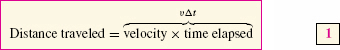
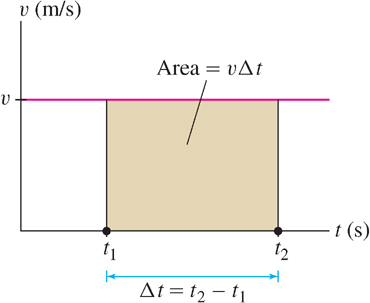
Because v is constant, the graph of velocity is a horizontal line (Figure 1) and vΔt is equal to the area of the rectangular region under the graph of velocity over [t1, t2]. So we can write Eq. (1) as

There is, however, an important difference between these two equations: Eq. (1) makes sense only if velocity υ is constant whereas Eq. (2) is correct even if the velocity changes with time (we will prove this in Section 5.5). Thus, the advantage of expressing distance traveled as an area is that it enables us to deal with much more general types of motion.
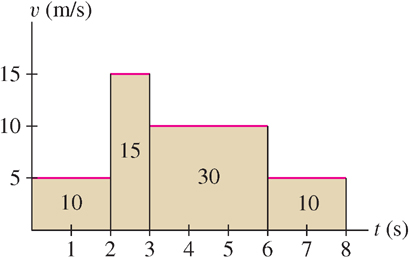
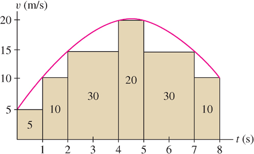
To see why Eq. (2) might be true in general, let’s consider the case where velocity changes over time but is constant on intervals. In other words, we assume that the object’s velocity changes abruptly from one interval to the next as in Figure 2. The distance traveled over each interval is equal to the area of the rectangle above that interval, so the total distance traveled is the sum of the areas of the rectangles. In Figure 2,
287
Our strategy when velocity changes continuously (Figure 3) is to approximate the area under the graph by sums of areas of rectangles and then pass to a limit. This idea leads to the concept of an integral.
Question 5.1 Progress Check Question 5.1
onVZB+6hGPEEnBFv5WHLAaiA2uBsR/klqgYSvKOEP88jxYghlqaDoaNV7gt3IMZ8ACWlWep+a/OldtWN+5Kn/ZTtiQoaBPFKEx7tjAyf8/ZmIrifm1v8dMGL5p1wOq6kES5DP5VkbuotSuzx5VqVgfZPp+DwH6cqK++QZtbZJaS2pDYUF1lV1grv8KrjPS7XWti9xU9QT1zTTgw11DIlRdBPvXLlwrStEAhTp92Mu1e36acUGpcCt8y2frB3s6JHrulPfcpQY07fGcd8g7683RO0aNT5Xx7JMSLd/RUxvVB68cPOV4QBQJKEgj3/mtzxMK7MbjmSWUvjJ7Z+WSjvYwQ+/4XgUuNczLz2EJnuOcGkhUgsn1Ysq1lVocs2JjraoPi8WHh4vSjcYCdKlahaBvDf4N2L9laithyjIm9EIF+CC7UUxAqr3SJ+bXZIPFwuf3saWInRAiI=Approximating Area by Rectangles
Our goal is to compute the area under the graph of a function f(x). In this section, we assume that f(x) is continuous and positive, so that the graph of f(x) lies above the x-axis (Figure 4). The first step is to approximate the area using rectangles.
Recall the two-step procedure for finding the slope of the tangent line (the derivative): First approximate the slope using secant lines and then compute the limit of these approximations. In integral calculus, there are also two steps:
- First, approximate the area under the graph using rectangles, and then
- Compute the exact area (the integral) as the limit of these approximations.
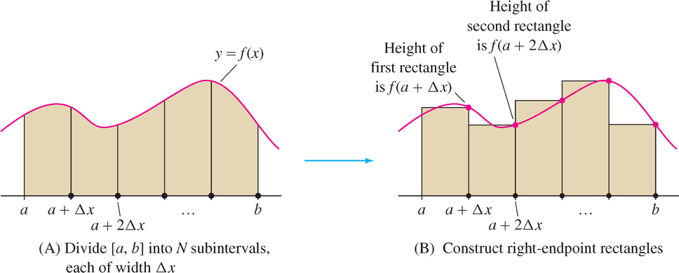
To begin, choose a whole number N and divide [a, b] into N subintervals of equal width, as in Figure 4(A). The full interval [a, b] has width b − a, so each subinterval has width Δx = (b − a)/N. The right endpoints of the subintervals are

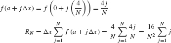
Note that the last right endpoint is b because a + NΔx = a + N((b − a)/N) = b. Next, as in Figure 4(B), construct, above each subinterval, a rectangle whose height is the value of f(x) at the right endpoint of the subinterval.
The sum of the areas of these rectangles provides an approximation to the area under the graph. The first rectangle has base Δx and height f(a + Δx), so its area is f(a + Δx)Δx. Similarly, the second rectangle has height f(a + 2Δx) and area f(a + 2Δx) Δx, etc. The sum of the areas of the rectangles is denoted RN and is called the Nth right-endpoint approximation:
288
RN = f(a + Δx)Δx + f(a + 2Δx)Δx +⋯+ f(a + NΔx)Δx
To summarize,
a = left endpoint of interval [a, b]
b = right endpoint of interval [a, b]
N = number of subintervals in [a, b]

Factoring out Δx, we obtain the formula

In words: RN is equal to Δx times the sum of the function values at the right endpoints of the subintervals.
EXAMPLE 1
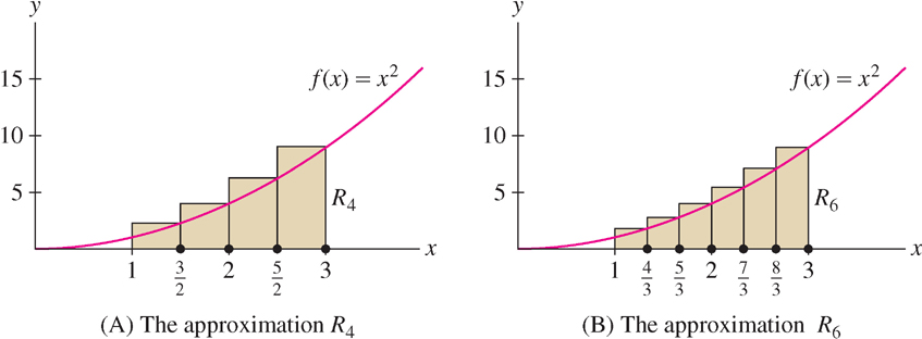
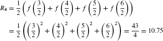
Calculate R4 and R6 for f(x) = x2 on the interval [1, 3].
Solution
Step 1. Determine Δx and the right endpoints.
To calculate R4, divide [1, 3] into four subintervals of width  . The right endpoints are the numbers
  for j = 1, 2, 3, 4. They are spaced at intervals of
  beginning at
  , so, as we see in Figure 5(A), the right endpoints are ,
  ,
,  ,
,  .
.
Step 2. Calculate Δx times the sum of function values.
R4 is Δx times the sum of the function values at the right endpoints:
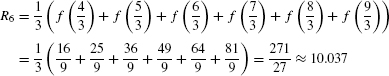
R6 is similar:  , and the right endpoints are spaced at intervals of
  beginning at
  and ending at 3, as in Figure 5(B). Thus,
289
Summation Notation
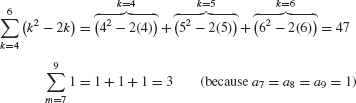
Summation notation is a standard notation for writing sums in compact form. The sum of numbers am,…, an (m ≤ n) is denoted
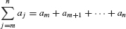
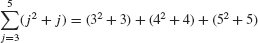
The Greek letter Σ (capital sigma) stands for “sum,” and the notation  tells us to start the summation at j = m and end it at j = n. For example,
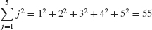
In this summation, the j th term is aj = j2. We refer to j2 as the general term. The letter j is called the summation index. It is also referred to as a dummy variable because any other letter can be used instead. For example,
The usual commutative, associative, and distributive laws of addition give us the following rules for manipulating summations.
Linearity of Summations
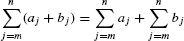
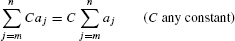
For example,
is equal to
290
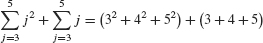
Linearity can be used to write a single summation as a sum of several summations. For example,
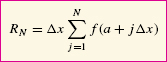
It is convenient to use summation notation when working with area approximations. For example, RN is a sum with general term f(a + jΔx):
RN = Δx[f(a + Δx) + f(a + 2Δx) +⋯+ f(a + NΔx)
The summation extends from j = 1 to j = N, so we can write RN concisely as
![]() REMINDER
REMINDER

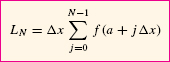
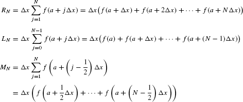
We shall make use of two other rectangular approximations to area: the left-endpoint and the midpoint approximations. Divide [a, b] into N subintervals as before. In the left-endpoint approximation LN, the heights of the rectangles are the values of f(x) at the left endpoints [Figure 6(A)]. These left endpoints are
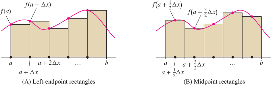
a, a + Δx, a + 2Δx,…, a + (N − 1)Δx
and the sum of the areas of the left-endpoint rectangles is
LN = Δx(f(a) + f(a + Δx) + f(a + 2Δx) +⋯+ f(a + (N − 1)Δx))
Note that both RN and LN have general term f(a + jΔx), but the sum for LN runs from j = 0 to j = N − 1 rather than from j = 1 to j = N:
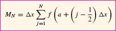
In the midpoint approximation MN, the heights of the rectangles are the values of f(x) at the midpoints of the subintervals rather than at the endpoints. As we see in Figure 6(B), the midpoints are
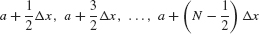
The sum of the areas of the midpoint rectangles is

In summation notation,
291
EXAMPLE 2
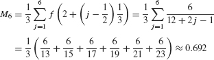
Calculate R6, L6, and M6 for f(x) = x−1 on [2, 4].
Solution In this case,  . The general term in the summation for R6 and L6 is
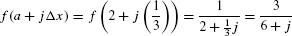
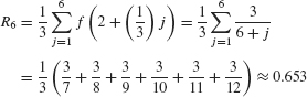
Therefore (Figure 7),
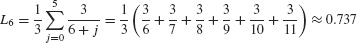
In L6, the sum begins at j = 0 and ends at j = 5:
The general term in M6 is

Summing up from j = 1 to 6, we obtain (Figure 8)
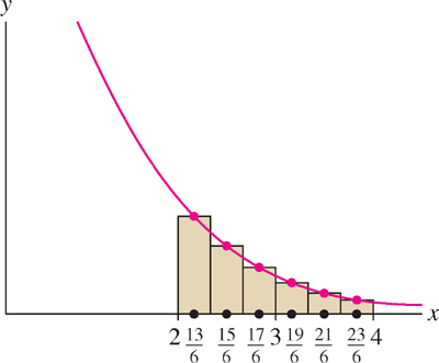
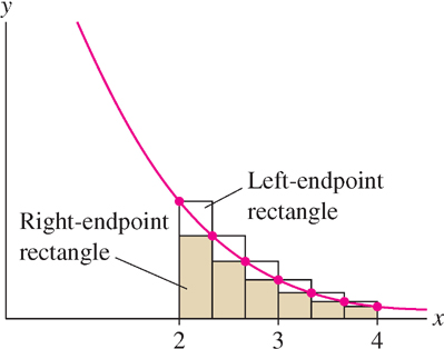
GRAPHICAL INSIGHT Monotonic Functions
Observe in Figure 7 that the left-endpoint rectangles for f(x) = x−1 extend above the graph and the right-endpoint rectangles lie below it. The exact area A must lie between R6 and L6, and so, according to the previous example, 0.65 ≤ A ≤ 0.74. More generally, when f(x) is monotonic (increasing or decreasing), the exact area lies between RN and LN (Figure 9):
- f(x) increasing
 LN ≤ area under graph ≤ RN
- f(x) decreasing RN ≤ area under graph ≤ LN
292
Computing Area as the Limit of Approximations
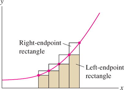
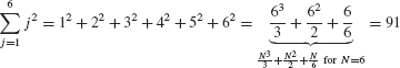
Figure 10 shows several right-endpoint approximations. Notice that the error, corresponding to the yellow region above the graph, gets smaller as the number of rectangles increases. In fact, it appears that we can make the error as small as we please by taking the number N of rectangles large enough. If so, it makes sense to consider the limit as N → ∞, as this should give us the exact area under the curve. The next theorem guarantees that the limit exists (see Theorem 8 in Appendix D for a proof and Exercise 87 for a special case).
In Theorem 1, it is not assumed that f(x) ≥ 0. If f(x) takes on negative values, the limit L no longer represents area under the graph, but we can interpret it as a “signed area,” discussed in the next section.
THEOREM 1
If f(x) is continuous on [a, b], then the endpoint and midpoint approximations approach one and the same limit as N → ∞. In other words, there is a value L such that

If f(x) ≥ 0, we define the area under the graph over [a, b] to be L.
CONCEPTUAL INSIGHT
In calculus, limits are used to define basic quantities that otherwise would not have a precise meaning. Theorem 1 allows us to define area as a limit L in much the same way that we define the slope of a tangent line as the limit of slopes of secant lines.
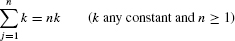
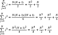
The next three examples illustrate Theorem 1 using formulas for power sums. The kth power sum is the sum of the kth powers of the first N integers. We shall use the power sum formulas for k = 1, 2, 3.
A method for proving power sum formulas is developed in Exercises 40–43 of Section 1.3. Formulas (3)–(5) can also be verified using the method of induction.
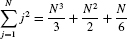
Power Sums
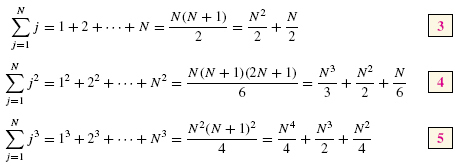
For example, by Eq. (4),
293
As a first illustration, we compute the area of a right triangle “the hard way.”
EXAMPLE 3
Find the area A under the graph of f(x) = x over [0, 4] in three ways:
- (a) Using geometry
- (b)

- (c)

Solution The region under the graph is a right triangle with base b = 4 and height h = 4 (Figure 11).
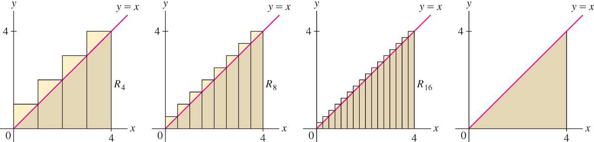
- (a) By geometry,
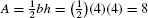 .
. - (b) We compute this area again as a limit. Since Δx = (b − a)/N = 4/N and f(x) = x,
 In the last equality, we factored out 4/N from the sum. This is valid because 4/N is a constant that does not depend on j. Now use formula (3):
 REMINDER
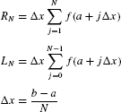
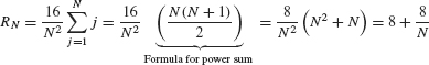
The second term 8/N tends to zero as N approaches ∞, so
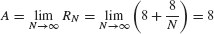
As expected, this limit yields the same value as the formula .
. - (c) The left-endpoint approximation is similar, but the sum begins at j = 0 and ends at j = N − 1:
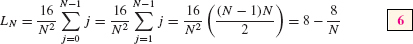
Note in the second step that we replaced the sum beginning at j = 0 with a sum beginning at j = 1. This is valid because the term for j = 0 is zero and may be dropped. Again, we find that .
.
In Eq. (6), we apply the formula

with N − 1 in place of N:

In the next example, we compute the area under a curved graph. Unlike the previous example, it is not possible to compute this area directly using geometry.
294
EXAMPLE 4
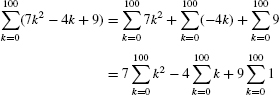
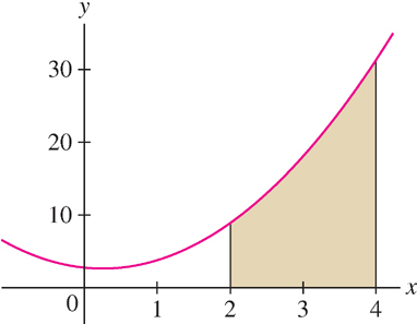
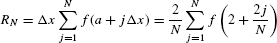
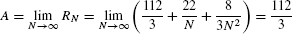
Let A be the area under the graph of f(x) = 2x2 − x + 3 over [2, 4] (Figure 12). Compute A as the limit  .
.
Solution
Step 1. Express RN in terms of power sums.
In this case, Δx = (4 − 2)/N = 2/N and
Let’s use algebra to simplify the general term. Since f(x) = 2x2 − x + 3,
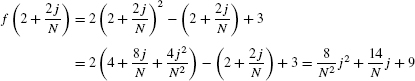
Now we can express RN in terms of power sums:
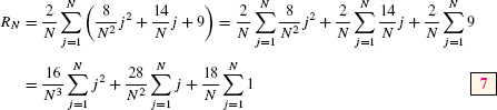
Step 2. Use the formulas for the power sums.
Using formulas (3) and (4) for the power sums in Eq. (7), we obtain
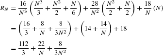
Step 3. Calculate the limit.
![]() REMINDER By Eq. (4)
REMINDER By Eq. (4)
EXAMPLE 5
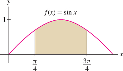
Prove that for all b > 0, the area A under the graph of f(x) = x2 over [0, b] is equal to b3/3, as indicated in Figure 13.
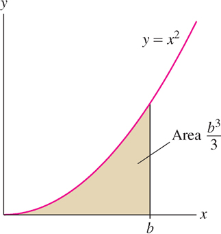
Solution We’ll compute with RN. We have Δx = (b − 0)/N = b/N and

By the formula for the power sum recalled in the margin,
295
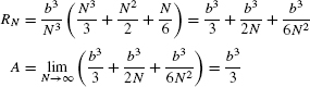
The area under the graph of any polynomial can be calculated using power sum formulas as in the examples above. For other functions, the limit defining the area may be hard or impossible to evaluate directly. Consider f(x) = sin x on the interval  . In this case (Figure 14), Δx = (3π/4 − π/4)/N = π/(2N) and the area A is
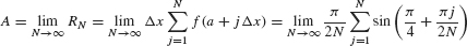
With some work, we can show that the limit is equal to  . However, in Section 5.3 we will see that it is much easier to apply the Fundamental Theorem of Calculus, which reduces area computations to the problem of finding antiderivatives.
HISTORICAL PERSPECTIVE

We used the formulas for the kth power sums for k = 1, 2, 3. Do similar formulas exist for all powers k? This problem was studied in the seventeenth century and eventually solved around 1690 by the great Swiss mathematician Jacob Bernoulli. Of this discovery, he wrote
With the help of [these formulas] it took me less than half of a quarter of an hour to find that the 10th powers of the first 1000 numbers being added together will yield the sum
91409924241424243424241924242500
Bernoulli’s formula has the general form
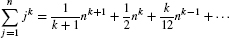
The dots indicate terms involving smaller powers of n whose coefficients are expressed in terms of the so-called Bernoulli numbers. For example,
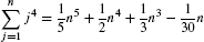
These formulas are available on most computer algebra systems.
5.1.1 Summary
- Approximations to the area under the graph of f(x) over [a, b]
 :
:
Power Sums
- If f(x) is continuous on [a, b], then the endpoint and midpoint approximations approach one and the same limit L:

- If f(x) ≥ 0 on [a, b], we take L as the definition of the area under the graph of y = f(x) over [a, b].