5.3 Antiderivatives and The Fundamental Theorem of Calculus, Part I
In addition to finding derivatives, there is an important “inverse” problem: Given the derivative, find the function itself. For example, in physics we may know the velocity \(v(t)\) (the derivative) and wish to compute the position \(s(t)\) of an object. Since \(s'(t) = v(t)\), this amounts to finding a function whose derivative is \(v(t)\). A function \(F(x)\) whose derivative is \(f(x)\) is called an antiderivative of \(f(x)\).
DEFINITION Antiderivatives
A function \(F(x)\) is an antiderivative of \(f(x)\) on \((a, b)\) if \(F'(x) = f(x)\) for all \(x \in (a, b)\).
Examples:
- \(F(x) = -\cos x\) is an antiderivative of \(f(x) = \sin x\) because
\[ F'(x) = \frac{d}{dx}(-\cos x) = \sin x = f(x) \]
- \(F(x)=\frac{1}{3}x^3\) is an antiderivative of \(f(x) = x^{2}\) because
\[ F'(x) = \frac{d}{dx}\left(\frac{1}{3}x^3\right) = x^2=f(x) \]
One critical observation is that antiderivatives are not unique. We are free to add a constant \(C\) because the derivative of a constant is zero, and so, if \(F'(x) = f(x)\), then \((F(x) + C)' = f(x)\). For example, each of the following is an antiderivative of \(x^{2}\):
\[ \frac{1}{3}x^3,\quad \frac{1}{3}x^3+5,\quad \frac{1}{3}x^3-4 \]
Are there any antiderivatives of \(f(x)\) other than those obtained by adding a constant to a given antiderivative \(F(x)\)? Our next theorem says that the answer is no if \(f(x)\) is defined on an interval \((a, b)\).
THEOREM 1 The General Antiderivative
Let \(F(x)\) be an antiderivative of \(f(x)\) on \((a, b)\). Then every other antiderivative on \((a, b)\) is of the form \(F(x) + C\) for some constant \(C\).
Proof
If \(G(x)\) is a second antiderivative of \(f(x)\), set \(H(x) = G(x) - F(x)\). Then \[ H'(x) = G'(x) - F'(x) = f(x) - f(x) = 0. \] Therefore \(H(x)\) must be a constant—say, \(H(x) = C\) —and therefore \(G(x) = F(x) + C\).
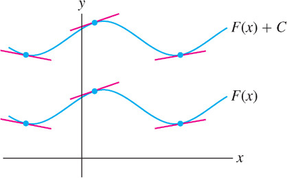
GRAPHICAL INSIGHT
The graph of \(F(x) + C\) is obtained by shifting the graph of \(F(x)\) vertically by \(C\) units. Since vertical shifting moves the tangent lines without changing their slopes, it makes sense that all of the functions \(F(x) + C\) have the same derivative (Figure 5.28). Theorem 1 tells us that conversely, if two graphs have parallel tangent lines, then one graph is obtained from the other by a vertical shift.
We often describe the general antiderivative of a function in terms of an arbitrary constant \(C\), as in the following example.
276
Example 1
Find two antiderivatives of \(f(x) = \cos x\). Then determine the general antiderivative.
Solution The functions \(F(x) = \sin x\) and \(G(x) = \sin x + 2\) are both antiderivatives of \(f(x)\). The general antiderivative is \(F(x) = \sin x + C\), where \(C\) is any constant.
Question 5.12 Antiderivative Progress Check Question 1
DGa+x0YQzXajJH7cdpTn6aWtYQA1OjlhEuTZBbcTEhFfAxXbDhNegOOHUQfa/klqdgSXbyor8gxEy8Il/PE547JpEp03bXxHwjpReJ83+B/ehDF2pFFa9spnuyd+mrBEI5lFXTUS0eCMlT2COeX4rHxKqOrhKGkTWMe3tem8Gts5LvhVfs9tBSeqM3blqBv7cY7KV3kIWA0=Why are we interested in finding antiderivatives? Well, the Fundamental Theorem of Calculus (FTC in short) connects the concept of antiderivative with that of area. The theorem has two parts. Although they are closely related, we discuss them in separate sections to emphasize the different ways they are used.
To explain FTC I, recall a result from Example 5 of Section 5.2: \[ \int\limits_4^7 x^2 dx = \left(\frac13\right)7^3 - \left(\frac13\right)4^3 = 93 \]
Now observe that \(F(x) = \left(\frac13\right)x^3\) is an antiderivative of \(x^2\), so we can write \[ \int\limits_4^7 x^2 dx = F(7) - F(4) \] According to FTC I, this is no coincidence; this relation between the definite integral and the antiderivative holds in general.
310
THEOREM 2 The Fundamental Theorem of Calculus, Part I
Assume that \(f(x)\) is continuous on \([a,b]\). If \(F(x)\) is an antiderivative of \(f(x)\) on \([a,b]\), then \[ \boxed{\bbox[#FAF8ED,5pt]{\int\limits_a^b f(x) \ dx = F(b) - F(a)} }\tag{1} \]
\(F(x)\) is called an antiderivative of \(f(x)\) if \(F'(x) = f(x)\).
The FTC was first stated clearly by Isaac Newton in 1666, although other mathematicians, including Newton’s teacher Isaac Barrow, had discovered versions of it earlier.
Proof
The quantity \(F(b)- F(a)\) is the total change in \(F\) (also called the “net change”) over the interval \([a,b]\). Our task is to relate it to the integral of \(F'(x) = f(x)\). There are two main steps.
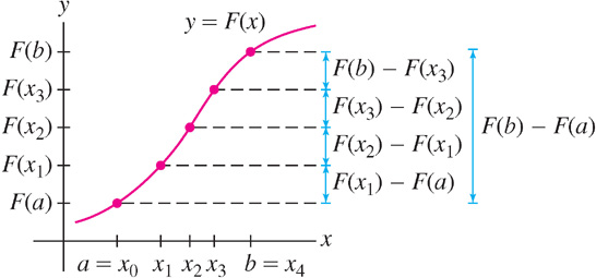
Step 1. Write total change as a sum of small changes.
Given any partition \(P\) of \([a,b]\) into \(N\) equal parts: \[ P\colon x_0=a < x_1 < x_2 < \cdots < x_N = b \] We can break up \(F(b) - F(a)\) as a sum of changes over the intervals \([x_{i-1},x_i]\): \[ F(b) - F(a) = \left( F(x_1) - F(a)\right) + \left( F(x_2) - F(x_1)\right) + \cdots + \left( F(b) - F(x_{N-1})\right) \] On the right-hand side, \(F(x_1)\) is canceled by \(- F(x_1)\) in the second term, \(F(x_2)\) is canceled by \(-F(x_2)\), etc. (Figure 5.29). In summation notation, \[ F(b) - F(a) = \sum\limits_{i=1}^N \left( F(x_i) - F(x_{i-1})\right)\tag{2} \]
Step 2. Interpret Eq. (2) as a Riemann sum.
The Mean Value Theorem tells us that there is a point \(x_i^*\) in \([x_{i-1},x_i]\) such that \[ F(x_i) - F(x_{i-1}) = F'(x_i^*)(x_i - x_{i-1}) = f(x_i^*)(x_i - x_{i-1}) = f(x_i^*)\Delta x_i \] Therefore, Eq. (2) can be written \[ F(b) - F(a) = \sum\limits_{i=1}^N f(x_i^*)\Delta x_i \] This sum is the Riemann sum \(\mbox{Rie}_N(f,X^*)\) with sample points \(X^* = \left\{x_i^*\right\}\).
Now, \(f(x)\) is integrable (Theorem 1, Section 5.2), so \(\mbox{Rie}_N(f,X^*)\) approaches \(\int_a^bf(x) dx\) as \(N\) tends to infinity. On the other hand, \(\mbox{Rie}_N(f,X^*)\) is equal to \(F(b) - F(a)\) with our particular choice \(X^*\) of sample points. This proves the desired result: \[ F(b) - F(a) = \lim\limits_{N \rightarrow \infty} \mbox{Rie}_N(f,X^*) = \int\limits_a^b f(x) dx \]
311
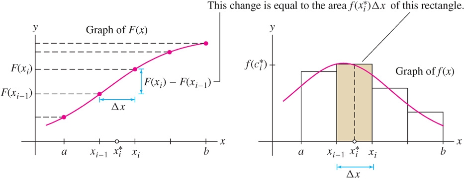
CONCEPTUAL INSIGHT A Tale of Two Graphs
In the proof of FTC I, we used the MVT to write a small change in \(F(x)\) in terms of the derivative \(F'(x) = f(x)\): \[ F(x_i) - F(x_{i-1}) = f(c_i^*)\Delta x_i \] But \(f(c_i^*)\Delta x_i\) is the area of a thin rectangle that approximates a sliver of area under the graph of \(f(x)\) (Figure 5.30). This is the essence of the Fundamental Theorem: the total change \(F(b) -F(a)\) is equal to the sum of small changes \(F(x_{i}) -F(x_{i-1})\), which in turn is equal to the sum of the areas of rectangles in a Riemann sum approximation for \(f(x)\). We derive the Fundamental Theorem itself by taking the limit as the width of the rectangles tends to zero.
FTC I tells us that if we can find an antiderivative of \(f(x)\), then we can compute the definite integral easily, without calculating any limits of Riemann sums.
Notation
\(F(b) -F(a)\) is denoted \(F(x)\Big|_a^b\). In this notation, the FTC reads \[ \int\limits_a^b f(x)dx = F(x)\bigg|_a^b \]
![]() REMINDER
The Power Rule for Integrals (valid for \(n \neq -1\)) states:
\[
\int x^ndx = \frac{x^{n+1}}{n+1}+C
\]
REMINDER
The Power Rule for Integrals (valid for \(n \neq -1\)) states:
\[
\int x^ndx = \frac{x^{n+1}}{n+1}+C
\]
EXAMPLE 2
Calculate the area under the graph of \(f(x) = x^{3}\) over \([2, 4]\).
Solution Since \(F(x)=\frac14x^4\) is an antiderivative of \(f(x) = x^{3}\), FTC I gives us \[ \int\limits_2^4 x^3dx = F(4) - F(2) = \frac14x^4\bigg|_2^4 = \frac144^4 - \frac142^4 = 60 \]
Question 5.13 FTC Progress Check Question 1
D6zUjgChUQU0vaUxrlQfcnDMIu1S/GypG/QdVSVAThSqvGZG4r55VMBQeexLZyOaPCg/cxaknFomCDGTLmbLDegWeBUt/e9BX4ZthwHAbUI=EXAMPLE 3
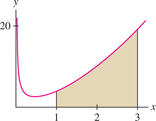
Find the area under \(g(x) = x^{-3/4} + 3x^{5/3}\) over \([1, 3]\)
Solution The function \(G(x) = 4x^{1/4} + \tfrac98x^{8/3}\) is an antiderivative of g(x). The area (Figure 5.31) is equal to \[ \begin{aligned} \int\limits_1^3 \left(x^{-3/4} + 3x^{5/3}\right)dx & = G(x)\bigg|_1^3 = \left(4x^{1/4} + \tfrac98x^{8/3}\right)\bigg|_1^3\\ & = \left(4\cdot3^{1/4} + \tfrac98\cdot3^{8/3}\right) - \left(4\cdot1^{1/4} + \tfrac98\cdot1^{8/3}\right)\\ & \approx 26.325 - 5.125 =21.1 \end{aligned} \]
312
EXAMPLE 4
Calculate \(\int_{-\pi/4}^{\pi/4}\sec^2x dx\) and sketch the corresponding region.
Solution Figure 5.32 shows the region. Recall that \((\tan x)' = \sec^{2}x\). Therefore,
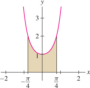
\[ \int\limits_{-\pi/4}^{\pi/4}\sec^2x dx = \tan x \bigg|_{-\pi/4}^{\pi/4} = \tan\left(\frac{\pi}{4}\right) - \tan\left(-\frac{\pi}{4}\right) = 1- (-1) = 2 \]
We know that the definite integral is equal to the sum and difference of areas of regions between the graph and the x-axis. Needless to say, the FTC “knows” this also: When you evaluate an integral using the FTC, you obtain the same sum and difference of these areas.
EXAMPLE 5
Evaluate
- (a) \(\int_0^{\pi} \sin x dx \)
and
- (b) \(\int_0^{2\pi} \sin x dx \).
Solution
- (a) Since \((-\cos x)' = \sin x\), the area of one “hump” (see Figure 5.33 below) is \[ \int\limits_0^{\pi} \sin x dx = -\cos x \bigg|_0^{\pi} = -\cos\pi - (-\cos 0) = - (-1) - (-1) = 2 \]
- (b) We expect the integral over \([0, 2\pi]\) to be zero since the second hump lies below the \(x\)-axis, and, indeed, \[ \int\limits_0^{2\pi} \sin x dx = -\cos x \bigg|_0^{2\pi} = -\cos2\pi - (-\cos 0) = - 1 - (-1) = 0 \]

Question 5.14 FTC Progress Check Question 2
8PGzNIVhyPG3FSl/o9Bhsoup2xH9kRmXIyqCeAR8Q/QfeJtprMiYRpm51u4FR0WlZcFLdZLkR3CRI9bUThe process of finding an antiderivative is called integration. We saw why in the connection between antiderivatives and areas under curves given by the Fundamental Theorem of Calculus. We now begin using the integral sign \(\int\) as the standard notation for antiderivatives.
NOTATION Indefinite Integral
The terms “antiderivative” and “indefinite integral” are used interchangeably. In some textbooks, an antiderivative is called a “primitive function.”
The notation
\[ \int f(x)dx = F(x) + C\quad\text{means that}\quad F'(x) = f(x) \]
We say that \(F(x) + C\) is the general antiderivative or indefinite integral of \(f(x)\).
The function \(f(x)\) appearing in the integral sign is called the integrand. The symbol \(dx\) is a differential. It is part of the integral notation and serves to indicate the independent variable. The constant \(C\) is called the constant of integration.
There are no Product, Quotient, or Chain Rules for integrals. However, we will see that the Product Rule for derivatives leads to an important technique called Integration by Parts (Section 7.1) and the Chain Rule leads to the Substitution Method (Section 5.6).
Some indefinite integrals can be evaluated by reversing the familiar derivative formulas. For example, we obtain the indefinite integral of \(x^{n}\) by reversing the Power Rule for derivatives.
THEOREM 3 Power Rule for Integrals
\[ \boxed{\bbox[#FAF8ED,5pt]{\displaystyle\int x^ndx = \frac{x^{n+1}}{n+1}+C\quad\text{for }n\neq -1}} \]
Proof
We just need to verify that \(F(x)=\dfrac{x^{n+1}}{n+1}\) is an antiderivative of \(f(x) = x^{n}\):
\[ F'(x)=\frac{d}{dx}\left(\frac{x^{n+1}}{n+1}\right) = \frac{1}{n+1}\left((n+1)x^n\right) = x^n \]
In words, the Power Rule for Integrals says that to integrate a power of \(x\), “add one to the exponent and then divide by the new exponent.” Here are some examples:
\[ \int x^5dx = \frac{1}{6}x^6 + C,\quad \int x^{-9}dx = -\frac{1}{8}x^{-8} + C,\quad \int x^{\frac{3}{5}}dx = \frac{5}{8}x^{\frac{8}{5}} + C \]
The Power Rule is not valid for \(n = -1\). In fact, for \(n = -1\), we obtain the meaningless result
\[ \int x^{-1}dx = \frac{x^0}{0} + C\quad\text{(meaningless)} \]
Notice that in integral notation, we treat dx as a movable variable, and thus we write \(\int\frac{1}{x}dx\) as \(\int\frac{dx}{x}\).
Recall, however, that the derivative of the natural logarithm is \(\frac{d}{dx}\ln x =\frac{1}{x}\). This shows that \(F(x) = \ln x\) is an antiderivative of \(y=\frac{1}{x}\). Thus, for \(n = -1\), instead of the Power Rule we have
\[ \int \frac{dx}{x} = \ln x + C \]
277
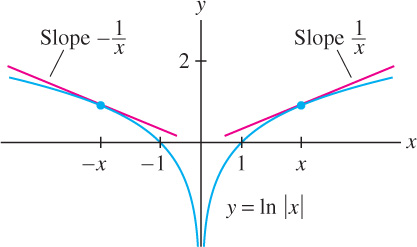
This formula is valid for \(x \gt 0\), where \(\ln x\) is defined. We would like to have an antiderivative of \(y=\frac{1}{x}\) on its full domain, namely on \(\{x : x \neq 0\}\). To achieve this end, we extend \(F(x)\) to an even function by setting \(F(x) = \ln |x|\) (Figure 5.34). Then \(F(x) = F(-x)\), and by the Chain Rule, \(F'(x) = -F'(-x)\). For \(x \lt 0\), we obtain
\[ \frac{d}{dx}\ln|x| = F'(x) = -F'(-x) = -\frac{1}{-x} = \frac{1}{x} \]
This proves that \(\frac{d}{dx}\ln|x|=\frac{1}{x}\) for all \(x \neq 0\).
THEOREM 4 Antiderivative of \(y=\frac{1}{x}\)
The function \(F(x) = \ln |x|\) is an antiderivative of \(y=\frac{1}{x}\) in the domain \(\{x : x \neq 0\}\); that is,
\[ \boxed{\bbox[#FAF8ED,5pt]{\displaystyle\int\frac{dx}{x} = \ln|x|+C}}\tag{3} \]
The indefinite integral obeys the usual linearity rules that allow us to integrate “term by term.” These rules follow from the linearity rules for the derivative.
THEOREM 5 Linearity of the Indefinite Integral
- Sum Rule: \(\displaystyle\int(f(x)+g(x))dx = \int f(x)dx + \int g(x)dx\)
- Scalar Multiples Rule: \(\displaystyle\int cf(x) dx = c\int f(x)dx\)
Example 6
Evaluate \(\displaystyle\int(3x^4-5x^{\frac{2}{3}}+x^{-3})dx\).
Solution We integrate term by term and use the Power Rule:
When we break up an indefinite integral into a sum of several integrals as in Example 2, it is not necessary to include a separate constant of integration for each integral.
\begin{align*} \int(3x^4-5x^{\frac{2}{3}}+x^{-3})dx &= \int 3x^4dx- \int 5x^{\frac{2}{3}}dx+ \int x^{-3}dx &&\text{(Sum Rule)}\\ &=3\int x^4dx- 5\int x^{\frac{2}{3}}dx+ \int x^{-3}dx &&\text{(Multiple Rule)}\\ &=3\left(\frac{x^5}{5}\right) - 5\left(\frac{x^{\frac{5}{3}}}{5/3}\right) + \frac{x^{-2}}{-2} + C &&\text{(Power Rule)}\\ &=\frac{3}{5}x^5 - 3x^{\frac{5}{3}} - \frac{1}{2}x^{-2} + C&& \end{align*}
To check the answer, we verify that the derivative is equal to the integrand:
\[ \frac{d}{dx}\left(\frac{3}{5}x^5 - 3x^{\frac{5}{3}} - \frac{1}{2}x^{-2} + C\right) = 3x^4-5x^{\frac{2}{3}}+x^{-3} \]
Example 7
Evaluate \(\displaystyle\int\left(\frac{5}{x}-3x^{-10}\right) \ dx\).
Solution Apply Eq. (3) and the Power Rule:
\begin{align*} \int\left(\frac{5}{x}-3x^{-10}\right) \ dx& = 5\int\frac{dx}{x} - 3\int x^{-10}dx\\ &=5\ln|x|-3\left(\frac{x^{-9}}{-9}\right) + C = 5\ln|x| + \frac{1}{3}x^{-9} +C \end{align*}
278
The differentiation formulas for the trigonometric functions give us the following integration formulas. Each formula can be checked by differentiation.
Basic Trigonometric Integrals
\begin{align*} \int\sin x \ dx &= -\cos x + C &\int\cos x \ dx &=\sin x+C\\ \int\sec^2x \ dx &= \tan x + C &\int\csc^2x \ dx&=-\cot x+C\\ \int\sec x\tan x \ dx&=\sec x+C &\int\csc x\cot x \ dx&=-\csc x+C\\ \end{align*}
Similarly, for any constants \(b\) and \(k\) with \(k \neq 0\), the formulas
\[ \frac{d}{dx}\sin(kx+b) = k\cos(kx+b)\quad \frac{d}{dx}\cos(kx+b) = -k\sin(kx+b) \]
translate to the following indefinite integral formulas:
\[\boxed{ \bbox[#FAF8ED,5pt]{\begin{aligned} \displaystyle\int\cos(kx+b) \ dx&=\dfrac{1}{k}\sin(kx+b) + C\\ \displaystyle\int\sin(kx+b) \ dx&=-\frac{1}{k}\cos(kx+b) + C \end{aligned}} }\]
Example 8
Evaluate \(\displaystyle\int \big(\sin(8t-3)+20\cos9t \big)dt\).
Solution
\begin{align*} \int \big(\sin(8t-3)+20\cos9t \big) \ dt &= \int\sin(8t-3) \ dt+20\int\cos9t \ dt\\ &=-\frac{1}{8}\cos(8t-3) + \frac{20}{9}\sin 9t + C \end{align*}
Question 5.15 Antiderivative Progress Check Question 2
XIed36ms0BYZubTgj2oVw5T+Aj2zko5Ns22eT/EkvUWVSK3uLzyfGfD9ArH3SDwzmvCrx+SOOT1iyN0MIzLyixNajrwvrCMGWrUQBEyX7B9ZIUZbLItQ2jO25jOZfvJewcd2tgEwy6VoOnZUz3OVPWmg/9RokUDk9XH03WILhZ8zFQ7kcrYuiRVe3BDQoFQhYm23TvHFWfyiuuGW+gEl5qe/HyOPNdccFwRk7BCkDyWYirwVMI07MQHKnZbcU5702T+fIeKqwTLa8xJ3W/ImWSiO5bGXbyR8qhoqcnOIOsACSbXjjil2jF3RUu4lw52KNYiMrd2/51RzU3F5Lnmib5e/tFkoJaXo6ifGyDnPEDnUl8cwVfc1473SCiIBO+JKDQtmO3iqQZU3/Y5jL7WglOkd9R8E6T9WoSVKT6Fuoli9dq+2edGkSgvaVaQSu0ZV/xq/Nd6gW03NcGgpNJ8o09CQs1fvnfK9XKMBwukaB8x4w2akpxIS41kTt4catMcG3++Xl6bd05Xv6jypabea+DaZgWHyQEuffdw6dzZeikpOZ+4Wk9W6a2M0jZ2CvRiAt4yLSdzD1Dsq2hQowtXlzP7ctWFOKQ4bY1Iry5wsnDwLcwOgRrRYmuLGLCKMjgpdcESCxnkdWvvQl8IiiuaS4XPafOUQxO5TZLbCmryULMQzEfgoYKO7v0EZcIwG2hOhnjEebVyDdOP/HBoo2QNcGuURpTqCt/JA313
CONCEPTUAL INSIGHT Which Antiderivative?
Antiderivatives are unique only to within an additive constant. Does it matter which antiderivative is used in the FTC? The answer is no. If \(F(x)\) and \(G(x)\) are both antiderivatives of \(f(x)\), then \(F(x) = G(x) + C\) for some constant \(C\), and \[ F(b) - F(a) = \underbrace{(G(b) + C) - (G(a) + C)}_{\text{The constant cancels}} = G(b) - G(a) \] The two antiderivatives yield the same value for the definite integral: \[ \int\limits_a^b f(x) dx = F(b) - F(a) = G(b) - G(a) \]
5.3.1 Summary
- \(F(x)\) is called an antiderivative of \(f(x)\) if \(F'(x) = f(x)\).
- Any two antiderivatives of \(f(x)\) on an interval \((a, b)\) differ by a constant.
- The general antiderivative is denoted by the indefinite integral
\[ \int f(x)dx = F(x) + C \]
- The Fundamental Theorem of Calculus, Part I, states that \[ \int\limits_a^b f(x)dx= F(b) - F(a) \] where \(F(x)\) is an antiderivative of \(f(x)\). FTC I is used to evaluate definite integrals in cases where we can find an antiderivative of the integrand.
- Basic antiderivative formulas for evaluating definite integrals: \[ \begin{array}{ll} \int x^n dx = \dfrac{x^{n+1}}{n+1} + C \text{ for }n\neq 1 & \\ \int e^x dx = e^x + C & \qquad\int \dfrac{dx}{x} = \ln |x| + C \\ \int \sin xdx = -\cos x + C & \qquad\int \cos xdx = \sin x + C \\ \int \sec^2x dx = \tan x + C & \qquad \int \csc^2x dx = -\cot x + C\\ \int \sec x\tan x dx = \sec x + C & \qquad\int\csc x \cot xdx= - \csc x + C\\ \int\sin(kx+b)dx=-\frac{1}{k}\cos(kx+b)+C (k\neq0) & \\ \int\cos(kx+b)dx= \frac{1}{k}\sin(kx+b)+C (k\neq0) & \\ \int e^{kx+b}dx=\frac{1}{k}e^{kx+b} + C (k\neq0)\\ \end{array} \]
314