2.2 The Geometry of Real-Valued Functions
76
We launch our investigation of real-valued functions by developing methods for visualizing them. In particular, we introduce the notions of a graph, a level curve, and a level surface of such functions.
Functions and Mappings
Let \(f\) be a function whose domain is a subset \(A\) of \({\mathbb R}^n\) and with a range contained in \({\mathbb R}^m\). By this we mean that to each \({\bf x}=(x_1,\ldots,x_n)\in A,f\) assigns a value \(f({\bf x})\), an \(m\)-tuple in \({\mathbb R}^m\). Such functions \(f\) are called vector-valued functionsfootnote # if \(m\,{>}\,1\), and scalar-valued functions if \(m=1\). For example, the scalar-valued function \(f(x,y,z)=(x^2+y^2+z^2)^{-3/2}\) maps the set \(A\) of \((x,y,z)\neq (0,0,0)\) in \({\mathbb R}^3\) (\(n=3\), in this case) to \({\mathbb R}\) \((m=1)\). To denote \(f\) we sometimes write \[ f\colon\, (x,y,z) \mapsto (x^2+y^2+z^2)^{-3/2}. \]
Note that in \({\mathbb R}^3\) we often use the notation \((x,y,z)\) instead of \((x_1,x_2,x_3)\). In general, the notation \({\bf x}\mapsto f({\bf x})\) is useful for indicating the value to which a point \({\bf x}\in {\mathbb R}^n\) is sent. We write \(f\colon A\subset {\mathbb R}^n \rightarrow {\mathbb R}^m\) to signify that \(A\) is the domain of \(f\)(a subset of \({\mathbb R}^n\)) and the range is contained in \({\mathbb R}^m\). We also use the expression \(f\) maps \(A\) into \({\mathbb R}^m\). Such functions \(f\) are called functions of several variables if \(A\subset {\mathbb R}^n, n > 1\).
As another example we can take the vector-valued function \(g\colon\, {\mathbb R}^6 \rightarrow {\mathbb R}^2\) defined by the rule \[ g({\bf x}) = g(x_1,x_2,x_3,x_4,x_5,x_6) = \Big(x_1x_2x_3x_4x_5x_6,{\textstyle\sqrt{x_1^2 + x_6^2}}\Big). \]
The first coordinate of the value of \(g\) at \({\bf x}\) is the product of the coordinates of \({\bf x}\).
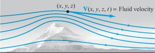
Functions from \({\mathbb R}^n\) to \({\mathbb R}^m\) are not just mathematical abstractions, they arise naturally in problems studied in all the sciences. For example, to specify the temperature \(T\) in a region \(A\) of space requires a function \(T \colon\, A\subset {\mathbb R}^3 \rightarrow {\mathbb R}\) \((n=3,m=1);\) thus, \(T(x,y,z)\) is the temperature at the point \((x,y,z)\). To specify the velocity of a fluid moving in space requires a map \({\bf V}\colon\, {\mathbb R}^4\rightarrow {\mathbb R}^3\), where \({\bf V}(x,y,z,t)\) is the velocity vector of the fluid at the point \((x,y,z)\) in space at time \(t\) (see Figure 2.1). To specify the reaction rate of a solution consisting of six reacting chemicals \(A,B, C,D,E,F\) in proportions \(x,y,z,w,u,v\) requires a map \(\sigma \colon\, U\subset {\mathbb R}^6\rightarrow {\mathbb R}\), where \(\sigma(x,y,z,w,u,v)\) gives the rate when the chemicals are in the indicated proportions.
77
To specify the cardiac vector (the vector giving the magnitude and direction of electric current flow in the heart) at time \(t\) requires a map \({\bf c}\colon\, {\mathbb R}\rightarrow {\mathbb R}^3, t \mapsto {\bf c} (t)\).
When \(f\colon\, U\subset {\mathbb R}^n\rightarrow {\mathbb R}\), we say that \(f\) is a real-valued function of n variables with domain U. The reason we say “\(n\) variables” is simply that we regard the coordinates of a point \({\bf x}=(x_1,\ldots,x_n)\in U\) as \(n\) variables, and \(f({\bf x})=f(x_1,\ldots,x_n)\) depends on these variables. We say “real-valued” because \(f(x_1,\ldots,x_n)\) is a real number. A good deal of our work will be with real-valued functions, so we give them special attention.
Graphs of Functions
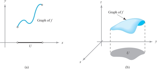
For \(f\colon\, U\subset {\mathbb R}\rightarrow {\mathbb R}\) \((n=1)\), the graph of \(f\) is the subset of \({\mathbb R}^2\) consisting of all points \((x,f(x))\) in the plane, for \(x\) in \(U\). This subset can be thought of as a curve in \({\mathbb R}^2\). In symbols, we write this as \[ \hbox{ graph} f = \{ (x, f(x)) \in {\mathbb R}^2 \mid x \in U\}, \] where the curly braces mean “the set of all” and the vertical bar is read “such that.” Drawing the graph of a function of one variable is a useful device to help visualize how the function actually behaves (see Figure 2.2). It will be helpful to generalize the idea of a graph to functions of several variables. This leads to the following definition:
Definition: Graph of a Function
Let \(f\colon\, U \subset {\mathbb R}^n \rightarrow {\mathbb R}\). Define the graph of \(f\) to be the subset of \(\,{\mathbb R}^{n+1}\) consisting of all the points \[ (x_1,\ldots,x_n, f(x_1,\ldots,x_n)) \] in \({\mathbb R}^{n+1}\) for \((x_1,\ldots,x_n)\) in \(U\). In symbols, \[ \hbox{ graph } f = \{(x_1,\ldots,x_n,f(x_1,\ldots,x_n)) \in {\mathbb R}^{n+1} \mid (x_1,\ldots,x_n)\in U\}. \]
For the case \(n=1\), the graph is a curve in \({\mathbb R}^2\), while for \(n=2\), it is a surface in \({\mathbb R}^3\) (see Figure 2.2). For \(n=3\), it is difficult to visualize the graph, because, since we are humans living in a three-dimensional world, it is hard for us to envisage sets in \({\mathbb R}^4\). To help overcome this handicap, we introduce the idea of a level set.
Level Sets, Curves, and Surfaces
78
Suppose \(f(x,y,z)= x^2 + y^2 + z^2\). A level set is a subset of \({\mathbb R}^3\) on which \(f\) is constant; for instance, the set where \(x^2+y^2+z^2= 1\) is a level set for \(f\). This we can visualize: It is just a sphere of radius 1 in \({\mathbb R}^3\). Formally, a level set is the set of \((x,y,z)\) such that \(f(x,y,z)=c\), where \(c\) is a constant. The behavior or structure of a function is determined in part by the shape of its level sets; consequently, understanding these sets aids us in understanding the function in question. Level sets are also useful for understanding functions of two variables \(f(x,y)\), in which case we speak of level curves or level contours.
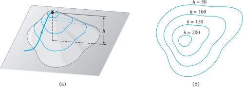
The idea is similar to that used to prepare contour maps, where one draws lines to represent constant altitudes; walking along such a line would mean walking on a level path. In the case of a hill rising from the \(xy\) plane, a graph of all the level curves gives us a good idea of the function \(h(x,y)\), which represents the height of the hill at point \((x,y)\) (see Figure 2.3).
example 1
The constant function \(f\colon\, {\mathbb R}^2 \rightarrow {\mathbb R}, (x,y)\mapsto 2\)—that is, the function \(f(x,y)=2\)—has as its graph the horizontal plane \(z=2\) in \({\mathbb R}^3\). The level curve of value \(c\) is empty if \(c\neq 2\), and is the whole \(xy\) plane if \(c=2\).
example 2
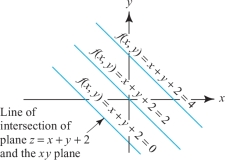
The function \(f\colon\, {\mathbb R}^2\rightarrow {\mathbb R},\) defined by \(f(x,y)=x+y+2\), has as its graph the inclined plane \(z=x+y+2\). This plane intersects the \(xy\) plane \((z=0)\) in the line \(y=-x-2\) and the \(z\) axis at the point \((0,0,2)\). For any value \(c \in {\mathbb R}\), the level curve of value \(c\) is the straight line \(y= - x+(c-2)\); or in symbols, the set \[ L_c = \{(x,y) \mid y = - x+ (c-2)\} \subset {\mathbb R}^2. \]
We indicate a few of the level curves of the function in Figure 2.4. This is a contour map of the function \(f\).
79
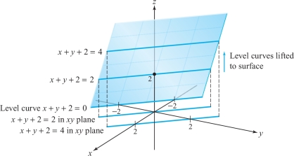
From level curves labeled with the value or “height” of the function, the shape of the graph may be inferred by mentally elevating each level curve to the appropriate height, without stretching, tilting, or sliding it. If this procedure is visualized for all level curves, \(L_c\)—that is, for all values \(c \in {\mathbb R}\), they will assemble to give the entire graph of \(f\), as indicated by the shaded plane in Figure 2.5. If the graph is visualized using a finite number of level curves, a contour model is produced. If \(f\) is a smooth function, its graph will be a smooth surface, and so the contour model, mentally smoothed over, gives a good impression of the graph.
Definition: Level Curves and Surfaces
Let \(f\colon\, U\subset {\mathbb R}^n \rightarrow {\mathbb R}\) and let \(c \in {\mathbb R}\). Then the level set of value \(c\) is defined to be the set of those points \({\bf x}\in U\) at which \(f({\bf x})=c\). If \(n=2\), we speak of a level curve (of value \(c\)); and if \(n=3\), we speak of a level surface. In symbols, the level set of value \(c\) is written \[ \{ {\bf x} \in U \mid f({\bf x}) = c \} \subset {\mathbb R}^n. \]
Note that the level set is always in the domain space.
example 3
Describe the graph of the quadratic function \[ f\colon \, {\mathbb R}^2\rightarrow {\mathbb R},(x,y) \mapsto x^2+y^2. \]
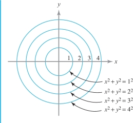
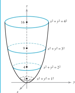
solution The graph is the paraboloid of revolution \(z=x^2+y^2\), oriented upward from the origin, around the \(z\) axis. The level curve of value \(c\) is empty for \(c<0\); for \(c>0\) the level curve of value \(c\) is the set \(\{(x,y) \mid x^2 + y^2 = c\}\), a circle of radius \(\sqrt{c}\) centered at the origin. Thus, raised to height \(c\) above the \(xy\) plane, the level set is a circle of radius \(\sqrt{c}\), indicating a parabolic shape (see Figure 2.6 and Figure 2.7).
80
The Method of Sections
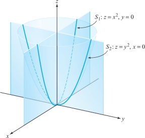
By a section of the graph of \(f\) we mean the intersection of the graph and a (vertical) plane. For example, if \(P_1\) is the \(xz\) plane in \({\mathbb R}^3\), defined by \(y=0\), then the section of \(f\) in Example 3 is the set \[ P_1 \cap \hbox{ graph } f = \{ (x,y,z) \mid y = 0,z=x^2 \}, \] which is a parabola in the \(xz\) plane. Similarly, if \(P_2\) denotes the \(yz\) plane, defined by \(x=0\), then the section \[ P_2 \cap \hbox{ graph } f = \{(x,y,z)\mid x=0, z=y^2 \} \] is a parabola in the \(yz\) plane (see Figure 2.8). It is usually helpful to compute at least one section to complement the information given by the level sets.
example 4
The graph of the quadratic function \[ f\colon\,{\mathbb R}^2 \rightarrow {\mathbb R}, (x,y) \mapsto x^2 \,{-}\,y^2 \] is called a hyperbolic paraboloid, or saddle, centered at the origin. Sketch the graph.
81
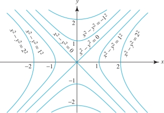
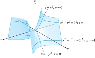
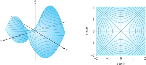
solution To visualize this surface, we first draw the level curves. To determine the level curves, we solve the equation \(x^2 - y^2= c\). Consider the values \(c=0, \pm 1, \pm 4\). For \(c=0\), we have \(y^2= x^2\), or \(y= \pm x\), so that this level set consists of two straight lines through the origin. For \(c=1\), the level curve is \(x^2-y^2=1\), or \(y=\pm \sqrt{x^2 -1},\) which is a hyperbola that passes vertically through the \(x\) axis at the points \((\pm 1,0)\) (see Figure 2.9). Similarly, for \(c=4\), the level curve is defined by \(y=\pm \sqrt{x^2-4}\), the hyperbola passing vertically through the \(x\) axis at \((\pm 2,0)\). For \(c=-1\), we obtain the curve \(x^2 - y^2 = -1\)—that is, \(x = \pm \sqrt{y^2-1}\)—the hyperbola passing horizontally through the \(y\) axis at \((0,\pm 1)\). And for \(c=-4\), the hyperbola through \((0,\pm 2)\) is obtained. These level curves are shown in Figure 2.9. Because it is not easy to visualize the graph of \(f\) from these data alone, we shall compute two sections, as in the previous example. For the section in the \(xz\) plane, we have \[ P_1 \cap \hbox{ graph of } f = \{ (x,y,z) \mid y=0,z=x^2\}, \] which is a parabola opening upward; and for the \(yz\) plane, \[ P_2 \cap \hbox{ graph } f = \{(x,y,z) \mid x=0, z=-y^2\}, \] which is a parabola opening downward. The graph may now be visualized by lifting the level curves to the appropriate heights and smoothing out the resulting surface. Their placement is aided by computing the parabolic sections. This procedure generates the hyperbolic saddle indicated in Figure 2.10. Compare this with the computer-generated graphs in Figure 2.11 (note that the orientation of the axes has been changed).
82
example 5
Describe the level sets of the function \[ f\colon\, {\mathbb R}^3 \rightarrow {\mathbb R}, (x,y,z)\mapsto x^2 + y^2 + z^2. \]
solution This is the three-dimensional analogue of Example 3. In this context, level sets are surfaces in the three-dimensional domain \({\mathbb R}^3\). The graph, in \({\mathbb R}^4\), cannot be visualized directly, but sections can nevertheless be computed.
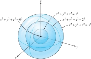
The level set with value \(c\) is the set \[ L_c = \{ (x,y,z) \mid x^2 + y^2 + z^2 = c\}, \] which is the sphere centered at the origin with radius \(\sqrt{c}\) for \(c>0\), is a single point at the origin for \(c=0\), and is empty for \(c<0\). The level sets for \(c=0,1,4\), and 9 are indicated in Figure 2.12.
83
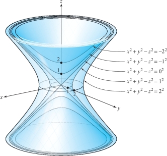
example 6
Describe the graph of the function \(f\colon\, {\mathbb R}^3 \rightarrow {\mathbb R}\) defined by \(f(x,y,z)=x^2+y^2-z^2,\) which is the three-dimensional analogue of Example 4, and is also called a saddle.
solution Formally, the graph of \(f\) is a subset of four-dimensional space. If we denote points in this space by \((x, y, z, t)\), then the graph is given by \[ \{(x, y, z, t)\mid t= x^2 + y^2 -z^2\}. \]
The level surfaces of \(f\) are defined by \[ L_c = \{(x,y,z) \mid x^2+ y^2 -z^2 = c\}. \]
For \(c=0\), this is the cone \(z= \pm \sqrt{x^2 + y^2}\) centered on the \(z\) axis. For \(c\) negative, say, \(c= -a^2\), we obtain \(z= \pm \sqrt{x^2 + y^2 + a^2}\), which is a hyperboloid of two sheets around the \(z\) axis, passing through the \(z\) axis at the points \((0, 0, \pm a)\). For \(c\) positive, say, \(c=b^2\), the level surface is the single-sheeted hyperboloid of revolution around the \(z\) axis defined by \(z= \pm \sqrt{x^2 + y^2- b^2}\), which intersects the \(xy\) plane in the circle of radius \(|b|\). These level surfaces are sketched in Figure 2.13.
84
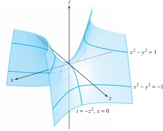
Another view of the graph may be obtained from a section. For example, the subspace \(S_{y=0}= \{(x,y,z,t)\mid y=0\}\) intersects the graph in the section \[ S_{y=0}\, \cap \hbox{ graph } f = \{ (x,y,z,t) \mid y=0,t=x^2 - z^2 \}, \] that is, the set of points of the form \((x,0,z,x^2 - z^2)\), which may be considered to be a surface in \(xzt\) space (see Figure 2.14).
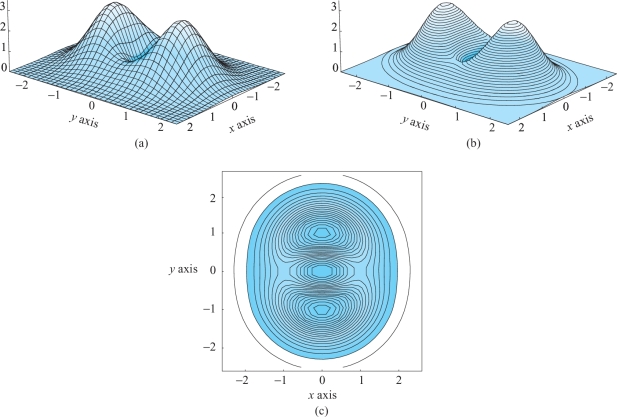
85
We have seen how the methods of sections and level sets can be used to understand the behavior of a function and its graph; these techniques can be quite useful to people who desire comprehensive visualization of complicated data. There are many computer programs available to do this, and we show the results of one such program in Figure 2.15.