3.5 Constrained Extrema and Lagrange Multipliers
Often we are required to maximize or minimize a function subject to certain constraints or side conditions. For example, we might need to maximize \(f(x, y)\) subject to the condition that \(x^2 + y^2 = 1\); that is, that \((x, y)\) lie on the unit circle. More generally, we might need to maximize or minimize \(f(x, y)\) subject to the side condition that \((x, y)\) also satisfies an equation \(g(x, y) =c\), where \(g\) is some function and \(c\) equals a constant [in the preceding example, \(g(x, y) = x^2 + y^2\), and \(c=1\)]. The set of such \((x, y)\) is a level curve for \(g\).
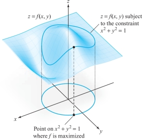
The purpose of this section is to develop some methods for handling this sort of problem. In Figure 3.14 we picture a graph of a function \(f(x, y)\). In this picture, the maximum of \(f\) might be at (0, 0). However, suppose we are not interested in this maximum but only the maximum of \(f(x, y)\) when \((x, y)\) belongs to the unit circle; that is, when \(x^2 + y^2 = 1\). The cylinder over \(x^2 + y^2 = 1\) intersects the graph of \(z = f(x, y)\) in a curve that lies on this graph. The problem of maximizing or minimizing \(f(x, y)\) subject to the constraint \(x^2 + y^2 = 1\) amounts to finding the point on this curve where \(z\) is the greatest or the least.
The Lagrange Multiplier Method
In general, let \(f {:}\, U \subset {\mathbb R}^n \rightarrow {\mathbb R}\) and \(g {:}\, U \subset {\mathbb R}^n \rightarrow {\mathbb R}\) be given \(C^1\) functions, and let \(S\) be the level set for \(g\) with value \(c\) [recall that this is the set of points \({\bf x} \in {\mathbb R}^n \) with \(g({\bf x}) = c\)].
186
When \(f\) is restricted to \(S\) we again have the notion of local maxima or local minima of \(f\) (local extrema), and an absolute maximum (largest value) or absolute minimum (smallest value) must be a local extremum. The following method provides a necessary condition for a constrained extremum:
Theorem 8 The Method of Lagrange Multipliers
Suppose that \(f {:}\,\, U \subset {\mathbb R}^n \rightarrow {\mathbb R}\) and \(g {:}\,\, U \subset {\mathbb R}^n \rightarrow {\mathbb R}\) are given \(C^1\) real-valued functions. Let \({\bf x}_0 \in U\) and \(g({\bf x}_0) = c\), and let \(S\) be the level set for \(g\) with value c [recall that this is the set of points \({\bf x} \in {\mathbb R}^n\) satisfying \(g({\bf x}) = c\)]. Assume \(\nabla\! g({\bf x}_0) \neq {\bf 0}\).
If \(f {\mid} S\), which denotes “\(f\) restricted to \(S\),” has a local maximum or minimum on \(S\) at \({\bf x}_0\), then there is a real number \(\lambda\) (which might be zero) such that \begin{equation*} \nabla\! f({\bf x}_0) = \lambda\! \nabla\! g({\bf x}_0).\tag{1} \end{equation*}
In general, a point \({\bf x}_0\) where equation (1) holds is said to be a critical point of \(f{\mid} S\).
proof
We have not developed enough techniques to give a complete proof, but we can provide the essential points. (The additional technicalities needed are discussed in Section 3.6 and in the Internet supplement.)
In Section 2.6 we learned that for \(n =3\) the tangent space or tangent plane of \(S\) at \({\bf x}_0\) is the space orthogonal to \(\nabla\! g({\bf x}_0)\). For arbitrary \(n\) we can give the same definition for the tangent space of \(S\) at \({\bf x}_0\). This definition can be motivated by considering tangents to paths \({\bf c}(t)\) that lie in \(S\), as follows: If \({\bf c}(t)\) is a path in \(S\) and \({\bf c}(0) = {\bf x}_0\), then \({\bf c}'(0)\) is a tangent vector to \(S\) at \({\bf x}_0\), but \[ \frac{d}{{\it dt}}g({\bf c}(t)) = \frac{d}{{\it dt}} c = 0, \] and, on the other hand, by the chain rule, \[ \frac{d}{{\it dt}}g({\bf c}(t)) \Big|_{t=0} =\nabla \!g({\bf x}_0) \,{\cdot}\, {\bf c}'(0), \] so that \(\nabla\! g({\bf x}_0) \,{\cdot}\, {\bf c}'(0)= 0\); that is, \({\bf c}' (0)\) is orthogonal to \(\nabla \! g({\bf x}_0)\).
If \(f {\mid} S\) has a maximum at \({\bf x}_0\), then \(f({\bf c}(t))\) has a maximum at \(t = 0\). By one-variable calculus, \(df ({\bf c}(t))/{\it dt}|_{t=0} = 0\). Hence, by the chain rule, \[ 0 = \frac{d}{{\it dt}}f({\bf c}(t))\Big|_{t=0} =\nabla \!f({\bf x}_0)\,{\cdot}\, {\bf c}'(0). \]
Thus, \(\nabla\! f ({\bf x}_0)\) is perpendicular to the tangent of every curve in \(S\) and so is perpendicular to the whole tangent space to \(S\) at \({\bf x}_0\). Because the space perpendicular to this tangent space is a line, \(\nabla\! f({\bf x}_0)\) and \(\nabla\! g({\bf x}_0)\) are parallel. Because \(\nabla \!g({\bf x}_0) \neq {\bf 0}\), it follows that \(\nabla \!f({\bf x}_0)\) is a multiple of \(\nabla\! g({\bf x}_0)\), which is the conclusion of the theorem.
Let us extract some geometry from this proof.
Theorem 9
If \(f\), when constrained to a surface \(S\), has a maximum or minimum at \({\bf x}_0\), then \(\nabla \! f({\bf x}_0)\) is perpendicular to \(S\) at \({\bf x}_0\) (see Figure 3.15).
187
These results tell us that in order to find the constrained extrema of \(f\), we must look among those points \({\bf x}_0\) satisfying the conclusions of these two theorems. We shall give several illustrations of how to use each.

When the method of Theorem 8 is used, we look for a point \({\bf x}_0\) and a constant \(\lambda\), called a Lagrange multiplier, such that \(\nabla\! f({\bf x}_0) = \lambda \! \nabla\! g({\bf x}_0)\). This method is more analytic in nature than the geometric method of Theorem 9. Surprisingly, Euler introduced these multipliers in 1744, some 40 years before Lagrange!
Equation (1) says that the partial derivatives of \(f\) are proportional to those of \(g\). Finding such points \({\bf x}_0\) at which this occurs means solving the simultaneous equations \begin{equation*} \left. \begin{array}{c} \\[-7pt] \displaystyle \frac{\partial f}{\partial x_1}(x_1,\ldots, x_n) = \lambda \displaystyle \frac{\partial g} {\partial x_1}(x_1, \ldots, x_n)\\[15pt] \displaystyle \frac{\partial f}{\partial x_2}(x_1,\ldots, x_n) = \lambda\displaystyle \frac{\partial g} {\partial x_2}(x_1, \ldots, x_n)\\[2.5pt] \vdots \\[2.5pt] \displaystyle \frac{\partial f}{\partial x_n}(x_1,\ldots, x_n) = \lambda \displaystyle \frac{\partial g} {\partial x_n}(x_1, \ldots, x_n)\\[13pt] g(x_1,\ldots, x_n) = c \\[3pt] \end{array} \right\}\tag{2} \end{equation*} for \(x_1,\ldots,x_n\) and \(\lambda\).
Another way of looking at these equations is as follows: Think of\(\lambda\) as an additional variable and form the auxiliary function \[ h(x_1,\ldots, x_n,\lambda) = f(x_1,\ldots, x_n) - \lambda[g(x_1, \ldots,x_n)-c] . \]
The Lagrange multiplier theorem says that to find the extreme points of \(f{\mid} S\), we should examine the critical points of \(h\). These are found by solving the equations \begin{equation*} \left. \begin{array}{l} 0 = \displaystyle \frac{\partial h}{\partial x_1} = \displaystyle \frac{\partial f}{\partial x_1} - \lambda \displaystyle \frac{\partial g}{\partial x_1}\\ \vdots\\ 0 = \displaystyle \frac{\partial h}{\partial x_n} = \displaystyle \frac{\partial f}{\partial x_n} - \lambda \displaystyle \frac{\partial g}{\partial x_n}\\[15pt] 0 = \displaystyle \frac{\partial h}{\partial \lambda} = g(x_1,\ldots, x_n) - c \end{array} \right\},\tag{3} \end{equation*} which are the same as equations (2) above.
188
Second-derivative tests for maxima and minima analogous to those in Section 3.4 will be given in Theorem 10 later in this section. However, in many problems it is possible to distinguish between maxima and minima by direct observation or by geometric means. Because this is often simpler, we consider examples of the latter type first.
example 1
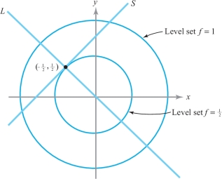
Let \(S\subset {\mathbb R}^2\) be the line through \((-1, 0)\) inclined at 45\(^\circ\), and let \(f{:}\,\, {\mathbb R}^2\rightarrow {\mathbb R},(x,y) \mapsto x^2 + y^2\). Find the extrema of \(f{\mid} S\).
solution Here \(S = \{(x, y)\mid y - x -1 = 0\}\), and therefore we set \(g(x, y) = y-x-1\) and \(c=0\). We have \({\nabla}\! g(x,y) = -{\bf i} + {\bf j} \neq {\bf 0}\). The relative extrema of \(f{|} S\) must be found among the points at which \({\nabla}\! f\) is orthogonal to \(S\); that is, inclined at \(-45^\circ\). But \(\nabla\! f(x, y) = (2x, 2y)\), which has the desired slope only when \(x = -y\), or when \((x,y)\) lies on the line \(L\) through the origin inclined at \(-45^\circ\). This can occur in the set \(S\) only for the single point at which \(L\) and \(S\) intersect (see Figure 3.16). Reference to the level curves of \(f\) indicates that this point, \((-{1}/{2}, {1}/{2})\), is a relative minimum of \(f{\mid} S\) (but not of \(f\)).
Notice that in this problem, \(f\) on \(S\) has a minimum but no maximum.
example 2
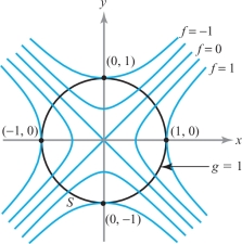
Let \(f{:}\,\, {\mathbb R}^2\rightarrow {\mathbb R},(x,y) \mapsto x^2 - y^2\), and let \(S\) be the circle of radius 1 around the origin. Find the extrema of \(f {\mid} S\).
solution The set \(S\) is the level curve for \(g\) with value 1, where \(g{:}\,\, {\mathbb R}^2\rightarrow {\mathbb R}, (x,y) \mapsto x^2 + y^2\). Because both of these functions have been studied in previous examples, we know their level curves; these are shown in Figure 3.17. In two dimensions, the condition that \({\nabla}\! f = \lambda\! {\nabla}\! g\) at \({\bf x}_0\)—that is, that \({\nabla}\! f\) and \(\nabla \!g\) are parallel at \({\bf x}_0\)—is the same as the level curves being tangent at \({\bf x}_0\) (why?). Thus, the extreme points of \(f{|}S\) are \((0, {\pm}1)\) and \(({\pm}1, 0)\). Evaluating \(f\), we find \((0, {\pm}1)\) are minima and \(({\pm}1, 0)\) are maxima.
Let us also do this problem analytically by the method of Lagrange multipliers. Clearly, \[ \nabla\! f(x, y) = \left(\frac{\partial f}{\partial x}, \frac{\partial f} {\partial y}\right) = (2x, - 2y)\quad \hbox{and} \quad {\nabla}\! g (x, y) = (2x, 2y). \]
189
Note that \({\nabla}\! g(x, y) \neq {\bf 0}\) if \(x^2 + y^2 = 1\). Thus, according to the Lagrange multiplier theorem, we must find a \(\lambda\) such that \[ (2x, -2y) = \lambda(2x,2y) \quad\hbox{and}\quad (x, y) \in S, \quad\hbox{i.e., } \ x^2 + y^2 =1. \]
These conditions yield three equations, which can be solved for the three unknowns \(x, y\), and \(\lambda\). From \(2x = \lambda 2x\), we conclude that either \(x=0\) or \(\lambda =1\). If \(x=0\), then \(y = {\pm}1\) and \(-2y = \lambda 2y\) implies \(\lambda =-1\). If \(\lambda =1\), then \(y=0\) and \(x = {\pm}1\). Thus, we get the points \((0, {\pm}1)\) and \(({\pm} 1, 0)\), as before. As we have mentioned, this method only locates potential extrema; whether they are maxima, minima, or neither must be determined by other means, such as geometric arguments or the second-derivative test given below.footnote #
example 3
Maximize the function \(f(x, y, z) = x+z\) subject to the constraint \(x^2 + y^2 +z^2 =1\).
solution By Theorem 7 we know that the function \(f\) restricted to the unit sphere \(x^2\,{+}\,y^2\,{+}\,z^2\,{=}\,1\) has a maximum (and also a minimum). To find the maximum, we again use the Lagrange multiplier theorem. We seek \(\lambda\) and \((x, y, z)\) such that \[ 1 = 2x\lambda,\qquad 0 = 2y\lambda, \quad \hbox{and} \quad 1 = 2z\lambda, \] and \[ x^2 + y^2 +z^2 =1. \]
From the first or the third equation, we see that \(\lambda \neq 0\). Thus, from the second equation, we get \(y=0\). From the first and third equations, \(x=z\), and so from the fourth, \(x = {\pm}1/\sqrt{2}=z\). Hence, our points are \((1/\sqrt{2}, 0, 1/\sqrt{2})\) and \((-1/\sqrt{2}, 0, -1/\sqrt{2})\). Comparing the values of \(f\) at these points, we can see that the first point yields the maximum of \(f\) (restricted to the constraint) and the second the minimum.
190
example 4
Assume that among all rectangular boxes with fixed surface area of 10 square meters there is a box of largest possible volume. Find its dimensions.
solution If \(\,x, y\), and \(z\) are the lengths of the sides, \(x \,{\geq}\, 0, y\,{\geq}\, 0, z\,{\geq}\, 0\), respectively, and the volume is \(f(x, y, z) =xyz\). The constraint is \(2(xy+xz + yz)=10\); that is, \(xy+xz+yz = 5\). Thus, the Lagrange multiplier conditions are \begin{eqnarray*} yz &=& \lambda (y+z)\\ xz &=& \lambda (x+z)\\ xy &=& \lambda (y+x)\\ xy + xz + yz &=& 5.\\[-17pt] \end{eqnarray*}
First of all, \(x \neq 0\), because \(x = 0\) implies \(yz = 5\) and \(0 = \lambda z\), so that \(\lambda = 0\) and we get the contradictory equation \(yz = 0\). Similarly, \(y\ne 0, z \ne 0, x+y\ne 0\). Elimination of \(\lambda\) from the first two equations gives \(yz/(y+z) =xz/(x+z)\), which gives \(x = y\); similarly, \(y = z\). Substituting these values into the last equation, we obtain \(3 x^2 = 5\), or \(x ={\sqrt{5/3}}\). Thus, we get the solution \(x = y = z= \sqrt{5/3}\), and \(xyz = (5/3)^{3/2}\). This (cubical) shape must therefore maximize the volume, assuming there is a box of maximum volume.
Existence of Solutions
We should note that the solution to Example 4 does not demonstrate that the cube is the rectangular box of largest volume with a given fixed surface area; it proves that the cube is the only possible candidate for a maximum. We shall sketch a proof that it really is the maximum later. The distinction between showing that there is only one possible solution to a problem and that, in fact, a solution exists is a subtle one that many (even great) mathematicians have overlooked.
Queen Dido (ca. 900 B.C.) realized that among all planar regions with fixed circumference, the disc is the region of maximum area. It is not difficult to prove this fact under the assumption that there is a region of maximum area; however, proving that such a region of maximum area exists is quite another (difficult) matter. A complete proof was not given until the second half of the nineteenth century by the German mathematician Weierstrass.
Let us consider a nonmathematical parallel to this situation. Put yourself in the place of Lord Peter Wimsey, Dorothy Sayers' famous detective:
“Undoubtedly,” said Wimsey, “but if you think that this identification is going to make life one grand, sweet song for you, you are mistaken\(\ldots\). Since we have devoted a great deal of time and thought to the case on the assumption that it was murder, it’s a convenience to know that the assumption is correct.”footnote #
Wimsey has found the body of a dead man, and after some time has located ten suspects. He is sure that no one else other than one of the suspects could be the murderer. By collecting all the evidence and checking alibis, he then reduces the number of suspects one by one, until, finally, only the butler remains; hence, he is the murderer! But wait, Peter is a very cautious man. By checking everything once again, he discovers that the man died by suicide; so there is no murder. You see the point: It does not suffice to find a clear and uniquely determined suspect in a criminal case where murder is suspected; you must prove that a murder actually took place.
The same goes for our cube; the fact that it is the only possible candidate for a maximum does not prove that it is maximum. (For more information see The Parsimonious Universe: Shape and Form in the Natural World, by S. Hildebrandt and A. Tromba, Springer-Verlag, New York/Berlin, 1995.)
191
The key to showing that \(f(x, y, z) = xyz\) really has a maximum lies in the fact that \(f\) is a continuous function that is defined on the unbounded surface \(S{:}\, xy + xz + yz = 5\), and not on a bounded set, which includes its boundary, where Theorem 7 of Section 3.4 would apply. We have already seen problems of this sort for functions of one and two variables.
The way to show that \(f(x, y, z) = xyz \ge 0\) does indeed have a maximum on \(xy + yz + xz = 5\) is to show that if \(x, y\), or \(z\) tend to \(\infty\), then \(f(x, y, z)\rightarrow 0\). We may then conclude that the maximum of \(f\) on \(S\) must exist by appealing to Theorem 7 (you should supply the details). So, suppose \((x, y, z)\) lies in \(S\) and \(x \to \infty\); then \(y \to 0\) and \(z \to 0\) (why?). Multiplying the equation defining \(S\) by \(z\), we obtain the equation \(xyz + xz^2 + yz^2 = 5z \to 0\) as \(x \to \infty\). Because \(x, y, z \ge 0, xyz = f(x, y, z) \to 0\). Similarly, \(f(x, y, z) \to 0\) if either \(y\) or \(z\) tend to \(\infty\). Thus, a box of maximum volume must exist.
Some general guidelines may be useful for maximum and minimum problems with constraints. First of all, if the surface \(S\) is bounded (as an ellipsoid is, for example), then \(f\) must have a maximum and a minimum on \(S\). (See Theorem 7 in the preceding section.) In particular, if \(f\) has only two points satisfying the conditions of the Lagrange multiplier theorems or Theorem 9, then one must be a maximum and one must be a minimum. Evaluating \(f\) at each point will tell the maximum from the minimum. However, if there are more than two such points, some can be saddle points. Also, if \(S\) is not bounded (for example, if it is a hyperboloid), then \(f\) need not have any maxima or minima.
Several Constraints
If a surface \(S\) is defined by a number of constraints, namely, \begin{equation*} \left. \begin{array}{l} g_1(x_1,\ldots,x_n) = c_1\\[2.5pt] g_2(x_1,\ldots,x_n) = c_2\\ \vdots\\[1pt] g_k(x_1,\ldots,x_n) = c_k \end{array}\right\},\tag{4} \end{equation*} then the Lagrange multiplier theorem may be generalized as follows: If \(f\) has a maximum or a minimum at \({\bf x}_0\) on \(S\), there must exist constants \(\lambda_1,\ldots,\lambda_k\) such thatfootnote # \begin{equation*} {\nabla}\! f({\bf x}_0) = \lambda_1\!{\nabla}\! g_1({\bf x}_0) + \cdots+\lambda_k {\nabla}\! g_k({\bf x}_0).\tag{5} \end{equation*}
This case may be proved by generalizing the method used to prove the Lagrange multiplier theorem. Let us give an example of how this more general formulation is used.
example 5
Find the extreme points of \(f(x, y, z) = x+ y+ z\) subject to the two conditions \(x^2 + y^2 = 2\) and \(x+z = 1\).
solution Here there are two constraints: \[ g_1(x, y, z) = x^2+y^2 - 2= 0\quad\hbox{and}\quad g_2(x, y, z) = x+ z -1 = 0. \]
192
Thus, we must find \(x, y, z, \lambda_1\), and \(\lambda_2\) such that \begin{eqnarray*} &{\nabla}\! f(x, y, z) = \lambda_1{\nabla}\! g_1(x, y, z) + \lambda_2{\nabla}\! g_2(x, y, z),&\\ &g_1(x, y, z) = 0,\quad \hbox{and}\quad g_2(x, y, z) = 0. & \\[-20pt] \end{eqnarray*}
Computing the gradients and equating components, we get \begin{eqnarray*} &\displaystyle 1 = \lambda_1 \,{\cdot}\, 2x+\lambda_2\,{\cdot}\, 1,\\ &\displaystyle 1 = \lambda_1 \,{\cdot}\, 2y+\lambda_2\,{\cdot}\, 0,\\ &\displaystyle 1 = \lambda_1 \,{\cdot}\, 0+\lambda_2\,{\cdot}\, 1,\\ &\displaystyle x^2 + y^2 = 2,\quad \hbox{and}\quad x + z = 1.\\[-20pt] \end{eqnarray*}
These are five equations for \(x, y, z, \lambda_1\), and \(\lambda_2\). From the third equation, \(\lambda_2=1\), and so \(2x\lambda_1 = 0, 2y\lambda_1=1\). Because the second implies \(\lambda_1 \ne 0\), we have \(x = 0\). Thus, \(y = {\pm}\sqrt{2}\) and \(z = 1\). Hence, the possible extrema are \((0, {\pm}\sqrt{2}, 1)\). By inspection, \((0,\sqrt{2},1)\) gives a relative maximum, and \((0, -\sqrt{2}, 1)\) a relative minimum.
The condition \(x^2 + y^2 = 2\) implies that \(x\) and \(y\) must be bounded. The condition \(x+z = 1\) implies that \(z\) is also bounded. If follows that the constraint set \(S\) is closed and bounded. By Theorem 7 it follows that \(f\) has a maximum and minimum on \(S\) that must therefore occur at \((0, \sqrt{2}, 1)\) and \((0, - \sqrt{2}, 1)\), respectively.
The method of Lagrange multipliers provides us with another tool to locate the absolute maxima and minima of differentiable functions on bounded regions in \({\mathbb R}^2\) (see the strategy for finding absolute maximum and minimum in Section 3.4).
example 6
Find the absolute maximum of \(f(x,y) = xy\) on the unit disc \(D\), where \(D\) is the set of points \((x, y)\) with \(x^2 + y^2 \le 1\).
solution By Theorem 7 in Section 3.4, we know the absolute maximum exists. First, we find all the critical points of \(f\) in \(U\), the set of points \((x, y)\) with \(x^2 + y^2 < 1\). Because \[ \frac{\partial f}{\partial x} = y \quad \hbox{and}\quad \frac{\partial f} {\partial y} = x, \] (0, 0) is the only critical point of \(f\) in \(U\). Now consider \(f\) on the unit circle, the level curve \(g(x, y) =1\), where \(g(x, y) = x^2 + y^2\). To locate the maximum and minimum of \(f\) on \(C\), we write down the Lagrange multiplier equations: \(\nabla\! f(x, y) = (y, x) = \lambda \!\nabla\! g(x, y) = \lambda (2x, 2y)\) and \(x^2 + y^2 = 1\). Rewriting these in component form, we get \begin{eqnarray*} y &=& 2\lambda x,\\ x &=& 2\lambda y,\\ x^2+y^2 &=& 1.\\[-19pt] \end{eqnarray*}
Thus, \[ y = 4 \lambda^2y, \] or \(\lambda = \pm 1/2\) and \(y = {\pm}x\), which means that \(x^2+x^2=2x^2=1\) or \(x = \pm {1}/{\sqrt{2}}, y = {\pm}{1}/{\sqrt{2}}\). On \(C\) we compute four candidates for the absolute maximum and minimum, namely, \[ \left( -\frac{1}{\sqrt{2}},-\frac{1}{\sqrt{2}}\right),\qquad \left( -\frac{1}{\sqrt{2}},\frac{1}{\sqrt{2}}\right),\qquad \left( \frac{1}{\sqrt{2}},\frac{1}{\sqrt{2}}\right),\qquad \left( \frac{1}{\sqrt{2}},-\frac{1}{\sqrt{2}}\right){.} \]
193
The value of \(f\) at both \((-1/\sqrt{2},-1/\sqrt{2})\) and \((1/\sqrt{2},1/\sqrt{2})\) is \(1/2\). The value of \(f\) at \(( -1/\sqrt{2},1/\sqrt{2})\) and \((1/\sqrt{2},-1/\sqrt{2})\) is \(-1/2\), and the value of \(f\) at (0, 0) is 0. Therefore, the absolute maximum of \(f\) is \(1/2\) and the absolute minimum is \(-1/2\), both occurring on \(C\). At \((0, 0), \partial^2\! f/ \partial x^2=0, \partial^2\! f/\partial y^2=0\) and \(\partial^2 \!f/\partial x\,\partial y=1\), so the discriminant is \(-1\) and thus (0, 0) is a saddle point.
example 7
Find the absolute maximum and minimum of \(f(x, y) = \frac{1}{2}x^2+\frac{1}{2}y^2\) in the elliptical region \(D\) defined by \(\frac{1}{2}x^2 + y^2 \le 1\).
solution Again by Theorem 7, Section 3.4, the absolute maximum exists. We first locate the critical points of \(f\) in \(U\), the set of points \((x, y)\) with \(\frac{1}{2}x^2 + y^2 < 1\). Because \[ \frac{\partial f}{\partial x} = x,\qquad \frac{\partial f}{\partial y} = y, \] the only critical point is the origin (0, 0).
We now find the maximum and minimum of \(f\) on \(C\), the boundary of \(U\), which is the level curve \(g(x, y) = 1\), where \(g(x, y) = \frac{1}{2}x^2 + y^2\). The Lagrange multiplier equations are \[ \nabla\! f(x, y) = (x, y) = \lambda\! \nabla\! g(x, y) = \lambda(x, 2y) \] and \((x^2/2) + y^2 = 1.\) In other words, \begin{eqnarray*} x &=& \lambda x\\[2pt] y &=& 2\lambda y\\[5pt] \frac{x^2}{2} + y^2 &=& 1. \end{eqnarray*}
If \(x = 0\), then \(y = {\pm}1\) and \(\lambda =\frac{1}{2}\). If \(y =0\), then \(x = {\pm}\sqrt{2}\) and \(\lambda =1\). If \(x \ne 0\) and \(y\ne 0\), we get both \(\lambda =1\) and \({1}/{2}\), which is impossible. Thus, the candidates for the maxima and minima of \(f\) on \(C\) are \((0, {\pm}1), ({\pm}\sqrt{2}, 0)\) and for \(f\) inside \(D\), the candidate is (0, 0). The value of \(f\) at \((0, {\pm}1)\) is \({1}/{2}\), at \(({\pm}\sqrt{2}, 0)\) it is 1, and at (0, 0) it is 0. Thus, the absolute minimum of \(f\) occurs at (0, 0) and is 0. The absolute maximum of \(f\) on \(D\) is thus 1 and occurs at the points \(({\pm}\sqrt{2}, 0)\).
Global Maxima and Minima
The method of Lagrange multipliers enhances our techniques for finding global maxima and minima. In this respect, the following is useful.
Definition
Let \(U\) be an open region in \({\mathbb R}^n\) with boundary \(\partial U\). We say that \(\partial U\) is smooth if \(\partial U\) is the level set of a smooth function \(g\) whose gradient \(\nabla\! g\) never vanishes (i.e., \(\nabla \! g\ne {\bf 0}\)). Then we have the following strategy.
194
Lagrange Multiplier Strategy for Finding Absolute Maxima and Minima on Regions with Boundary
Let \(f\) be a differentiable function on a closed and bounded region \(D = U \cup \partial U, U\) open in \({\mathbb R}^n\), with smooth boundary \(\partial U\).
To find the absolute maximum and minimum of \(f\) on \(D\):
- (i) Locate all critical points of \(f\) in \(U\).
- (ii) Use the method of Lagrange multiplier to locate all the critical points of \(f{\mid} \partial U\).
- (iii) Compute the values of \(f\) at all these critical points.
- (iv) Select the largest and the smallest.
example 8
Find the absolute maximum and minimum of the function \(f(x, y, z) = x^2+ y^2+ z^2-x+y\) on the set \(D = \{(x, y, z) \mid x^2+y^2+z^2 \le 1\}\).
solution As in the previous examples, we know the absolute maximum and minimum exists. Now \(D = U \cup \partial U\), where \[ U = \{(x, y, z) \mid x^2+y^2+z^2 < 1\} \] and \[ \partial U = \{(x, y, z) \,|\, x^2+y^2+z^2 = 1\}. \] \(\nabla \!f(x,y,z)=(2x-1, 2y+1, 2z)\).
Thus, \(\nabla f=0\) at \((1/2,-1/2,0)\) which is in \(U\), the interior of \(D\).
Let \(g(x, y, z) = x^2 + y^2 + z^2\). Then \(\partial U\) is the level set \(g(x, y, z)=1\). By the method of Lagrange multipliers, the maximum and minimum must occur at a critical point of \(f{|} \partial U\); that is, at a point \({\bf x}_0\) where \(\nabla\!\! f ({\bf x}_0) = \lambda\! \nabla g({\bf x}_0)\) for some scalar \(\lambda\).
Thus, \[ (2x-1,2y+1,2z)=\lambda (2x, 2y, 2z) \] or
- (i) \(2x-1=2\lambda x\)
- (ii) \(2y+1=2 \lambda y\)
(iii) \(2z=2\lambda z\)
If \(\lambda=1\), then we would have \(2x-1=2x\) or \(-1=0\), which is impossible. We may assume that \(\lambda \neq 0\) since if \(\lambda = 0\), we only get an interior point as above. Thus (iii) implies that \(z=0\) and
(iv) \(x^2+y^2=1\).
Solving (i) and (ii) for \(x\) and \(y\) we find,
- (v) \(x=1/2(1-\lambda)\)
- (vi) \(y=-1/2(1-\lambda)\)
195
Applying (iv) we can solve for \(\lambda\), namely \(\lambda=1\pm(1/\sqrt{2})\). Thus, from (v) and (vi) we have that \(x=\pm(1/\sqrt{2})\) and \(y=\pm(1/\sqrt{2})\); that is, we have four critical points on \(\partial U\). Evaluating \(f\) at each of these points, we see that the maximum value for \(f\) on \(\partial U\) is \(1+2/\sqrt{2}=1+\sqrt{2}\) and the minimum value is \(1-\sqrt{2}\). The value of \(f\) at \((1/2,-1/2)\) is \(-1/2\). Comparing these values, noting that \(-1/2<1-\sqrt{2}\), we see that the absolute minimum is \(-1/2\), occurring at \((1/2,-1/2)\), and that absolute maximum is \(1+\sqrt{2}\), occurring at \((-1/\sqrt{2},1/\sqrt{2})\).
Two Additional Applications
We now present two further applications of the mathematical techniques developed in this section to geometry and to economics. We shall begin wth a geometric example.
example
Suppose we have a curve defined by the equation \[ \phi(x,y) = Ax^2 + 2Bxy + Cy^2 -1 =0. \]
Find the maximum and minimum distance of the curve to the origin. (These are the lengths of the semimajor and the semiminor axis of this quadric.)
solution The problem is equivalent to finding the extreme values of \(f(x,y)=x^2 + y^2\) subject to the constraining condition \(\phi (x,y)=0\). Using the Lagrange multiplier method, we have the following equations: \begin{equation*} 2x + \lambda(2Ax + 2By) = 0\tag{6} \end{equation*} \begin{equation*} 2y + \lambda(2Bx + 2Cy) = 0\tag{7} \end{equation*} \begin{equation*} Ax^2 + 2Bxy + Cy^2 = 1 .\tag{8} \end{equation*}
Adding \(x\) times equation (6) to \(y\) times equation (7), we obtain \[ 2(x^2 + y^2) + 2\lambda(Ax^2 +2Bxy + Cy^2)=0. \]
By equation (8), it follows that \(x^2 + y^2 +\lambda =0\). Let \(t=-1/\lambda = 1/(x^2 + y^2)\) [the case \(\lambda =0\) is impossible, because (0, 0) is not on the curve \(\phi(x,y)=0]\). Then equations (6) and (7) can be written as follows: \begin{equation*} \begin{array}{c} 2(A-t)x + 2By =0\\[6pt] 2Bx + 2(C-t)y =0. \end{array}\tag{9} \end{equation*}
If these two equations are to have a nontrivial solution [remember that \((x,y)=(0,0)\) is not on our curve and so is not a solution], it follows from a theorem of linear algebra that their determinant vanishes:footnote # \[ \left | \begin{array}{c@{\quad}c} A-t & B\\ B & C-t \end{array}\right | =0. \]
Because this equation is quadratic in \(t\), there are two solutions, which we shall call \(t_1\) and \(t_2\). Because \(-\lambda = x^2 + y^2\), we have \({\sqrt{x^2 + y^2}} = {\sqrt{-\lambda}}\). Now \({\sqrt{x^2 + y^2}}\) is the distance from the point \((x,y)\) to the origin. Therefore, if \((x_1,y_1)\) and \((x_2,y_2)\) denote the nontrivial solutions to equation (9) corresponding to \(t_1\) and \(t_2\), and if \(t_1\) and \(t_2\) are positive, we get \({\textstyle \sqrt{{x_2^2 + y^2_2}}}= 1/{\textstyle\sqrt{t_2}}\) and \({\textstyle \sqrt{{x_1^2 + y^2_1}}}= 1/{\textstyle\sqrt{t_1}}\). Consequently, if \(t_1 >t_2\), the lengths of the semiminor and semimajor axes are \(1/\sqrt{t_1}\) and \(1/\sqrt{t_2}\), respectively. If the curve is an ellipse, both \(t_1\) and \(t_2\) are, in fact, real and positive. What happens with a hyperbola or a parabola?
196
Finally, we discuss an application to economics.
example
Suppose that the output of a manufacturing firm is a quantity \(Q\) of a certain product, where \(Q\) is a function \(f(K,L)\), where \(K\) is the amount of capital equipment (or investment) and \(L\) is the amount of labor used. If the price of labor is \(p,\) the price of capital is \(q,\) and the firm can spend no more than \(B\) dollars, how can we find the amount of capital and labor to maximize the output \(Q\)?
solution We would expect that if the amount of capital or labor is increased, then the output \(Q\) should also increase; that is, \[ \frac{\partial Q}{\partial K}\geq 0 \quad \hbox{and} \quad \frac{\partial Q}{\partial L}\geq 0. \]
We also expect that as more labor is added to a given amount of capital equipment, we get less additional output for our effort; that is, \[ \frac{\partial^2\! Q}{\partial L^2} < 0. \]
Similarly, \[ \frac{\partial^2\! Q}{\partial K^2} < 0. \]
With these assumptions on \(Q\), it is reasonable to expect the level curves of output (called isoquants) \(Q(K,L)=c\) to look something like the curves sketched in Figure 3.18, with \(c_1 < c_2 < c_3\).
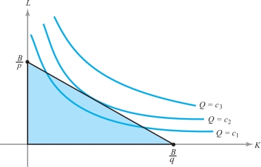
197
We can interpret the convexity of the isoquants as follows: As we move to the right along a given isoquant, it takes more and more capital to replace a unit of labor and still produce the same output. The budget constraint means that we must stay inside the triangle bounded by the axes and the line \(pL +qK =B\). Geometrically, it is clear that we produce the most by spending all our money in such a way as to pick the isoquant that just touches, but does not cross, the budget line.
Because the maximum point lies on the boundary of our domain, we apply the method of Lagrange multipliers to find the maximum. To maximize \(Q=f(K,L)\) subject to the constraint \(pL + qK =B\), we look for critical points of the auxiliary function, \[ h(K,L,\lambda) = f(K,L) -\lambda (pL + qK -B). \]
Thus, we want \[ \frac{\partial Q}{\partial K} =\lambda q,\qquad \frac{\partial Q}{\partial L} ={\lambda} p, \quad\hbox{and}\quad pL +qK =B. \]
These are the conditions we must meet in order to maximize output. (You are asked to work out a specific case in Exercise 36.)
In the preceding example, \(\lambda\) represents something interesting. Let \(k=qK\) and \(l = pL\), so that \(k\) is the dollar value of the capital used and \(l\) is the dollar value of the labor used. Then the first two equations become \[ \frac{\partial Q}{\partial k} =\frac{1}{q} \frac{\partial Q}{\partial K} = \lambda = \frac{1}{p} \frac{\partial Q}{\partial L}= \frac{\partial Q}{\partial l}. \]
Thus, at the optimum production point the marginal change in output per dollar’s worth of additional capital investment is equal to the marginal change of output per dollar’s worth of additional labor, and \(\lambda\) is this common value. At the optimum point, the exchange of a dollar’s worth of capital for a dollar’s worth of labor does not change the output. Away from the optimum point the marginal outputs are different, and one exchange or the other will increase the output.
A Second-Derivative Test for Constrained Extrema
In Section 3.4 we developed a second-derivative test for extrema of functions of several variables by looking at the second-degree term in the Taylor series of \(f\). If the Hessian matrix of second partial derivatives is either positive-definite or negative-definite at a critical point of \(f\), this point is a relative minimum or maximum, respectively.
The question naturally arises as to whether there is a second-derivative test for maximum and minimum problems in the presence of constraints. The answer is yes and the test involves a matrix called a bordered Hessian. We will first discuss the test and how to apply it for the case of a function \(f(x, y)\) of two variables subject to the constraint \(g(x, y)=c\).
198
Theorem 10
Let \(f\colon\, U \subset {\mathbb R}^2 \to {\mathbb R}\) and \(g\colon\, U \subset {\mathbb R}^2 \to {\mathbb R}\) be smooth (at least \(C^2\)) functions. Let \({\bf v}_0 \in U,\) \(g({\bf v}_0) =c\), and \(S\) be the level curve for \(g\) with value \(c\). Assume that \(\nabla\! g({\bf v}_0)\neq {\bf 0}\) and that there is a real number \(\lambda\) such that \({\nabla}\! f({\bf v}_0) = \lambda\! {\nabla}\!g({\bf v}_0)\). Form the auxiliary function \(h = f-\lambda g\) and the bordered Hessian determinant \[ |{\skew6\overline{H}}| = \left|\begin{array}{c@{\quad}c@{\quad}c} 0 & \displaystyle-\frac{\partial g}{\partial x} & \displaystyle - \frac{\partial g}{\partial y}\\[7pt] \displaystyle-\frac{\partial g}{\partial x} & \displaystyle \frac{\partial^2\! h}{\partial x^2} & \displaystyle \frac{\partial^2\! h}{\partial x\,\partial y}\\[7pt] \displaystyle -\frac{\partial g}{\partial y} & \displaystyle \frac{\partial^2h}{\partial x\,\partial y} & \displaystyle \frac{\partial^2h}{\partial y^2} \end{array}\right|\quad \hbox{evaluated at } {\bf v}_0. \]
- (i) If \(|{\skew6\overline{H}}| > 0,\) then \({\bf v}_0\) is a local maximum point for \(f{\mid} S\).
- (ii) If \(|{\skew6\overline{H}}| < 0,\) then \({\bf v}_0\) is a local minimum point for \(f| S\).
- (iii) If \(|{\skew6\overline{H}}| =0,\) the test is inconclusive and \({\bf v}_0\) may be a minimum, a maximum, or neither.
This theorem is proved in the Internet supplement for this section.
example 11
Find extreme points of \(f(x,y)= (x-y)^n\) subject to the constraint \(x^2 + y^2 = 1,\) where \(n \ge 1\).
solution We set the first derivatives of the auxiliary function \(h\) defined by \(h(x,y,\lambda) = (x-y)^n - \lambda (x^2\) \(+\) \(y^2 -1)\) equal to 0: \begin{eqnarray*} n(x-y)^{n-1} - 2\lambda x &=& 0\\ -n(x-y)^{n-1} - 2\lambda y &=& 0\\ -(x^2 + y^2 - 1) &=& 0.\\[-18pt] \end{eqnarray*}
From the first two equations we see that \(\lambda(x+y) =0\). If \(\lambda=0\), then \(x = y = \pm \sqrt{2}/2\). If \(\lambda \neq 0\), then \(x= - y\). The four critical points are represented in Figure 3.19, and the corresponding values of \(f(x,y)\) are listed below: \[ \begin{array}{lr@{\,}c@{\,}lr@{\,}c@{\,}lr@{\,}c@{\,}lr@{\,}c@{\,}l} {\rm (A)} & x &=&\sqrt{2}/2 & y &=&\sqrt{2}/2 & \lambda &=& 0 & f(x,y) &=& 0 \end{array} \]
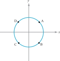
\[ \begin{array}{lr@{\,}c@{\,}lr@{\,}c@{\,}lr@{\,}c@{\,}lr@{\,}c@{\,}l} {\rm (B)} & x &=&\sqrt{2}/2 & y &=&-\sqrt{2}/2 & \lambda &=& n(\sqrt{2})^{n-2} & f(x,y) &=& (\sqrt{2})^n\\[5pt] {\rm (C)} & x &=& -\sqrt{2}/2 & y &=& -\sqrt{2}/2 & \lambda &=& 0 & f(x,y) &=& 0\\[5pt] {\rm (D)} & x &=&-\sqrt{2}/2 & y &=&\sqrt{2}/2 &\lambda &=& (-1)^{n-2}n(\sqrt{2})^{n-2} &f(x,y) &=& (-\sqrt{2})^n. \end{array} \]
199
By inspection, we see that if \(n\) is even, then A and C are minimum points and B and D are maxima. If \(n\) is odd, then B is a maximum point, D is a minimum, and A and C are neither. Let us see whether Theorem 10 is consistent with these observations.
The bordered Hessian determinant is \begin{eqnarray*} |{\skew6\overline{H}}| &=& \left|\begin{array}{c@{\quad}c@{\quad}c} 0 &-2x & -2y\\[2pt] -2x & n(n-1)(x-y)^{n-2}-2\lambda & - n(n-1)(x-y)^{n-2}\hphantom{-2\lambda aa.}\\[4pt] -2y & - n(n-1)(x-y)^{n-2}\hphantom{-2\lambda a.} & n(n-1)(x-y)^{n-2}-2\lambda\!\! \end{array}\!\!\right|\\[4pt] &=& -4n(n-1)(x-y)^{n-2} (x+y)^2 + 8\lambda(x^2 - y^2). \end{eqnarray*}
If \(n=1\) or if \(n \ge 3, |{\skew6\overline{H}}| = 0\) at A, B, C, and D. If \(n = 2\), then \(|{\skew6\overline{H}}|=0\) at B and D and \(-16\) at A and C. Thus, the second-derivative test picks up the minima at A and C, but is inconclusive in testing the maxima at B and D for \(n=2\). It is also inconclusive for all other values of \(n\).
Just as in the unconstrained case, there is also a second-derivative test for functions of more than two variables. If we are to find extreme points for \(f(x_1,\ldots,x_n)\) subject to a single constraint \(g(x_1,\ldots, x_n) = c\), we first form the bordered Hessian for the auxiliary function \(h(x_1,\ldots, x_n) = f(x_1,\ldots, x_n) - \lambda(g(x_1,\ldots, x_n)-c)\) as follows: \[ \left|\begin{array}{c@{\quad}c@{\quad}c@{\quad}c@{\quad}c} 0 &\displaystyle\frac{-\partial g}{\partial x_1} &\displaystyle\frac{-\partial g}{\partial x_2} &\cdots & \displaystyle\frac{-\partial g}{\partial x_n}\\[12pt] \displaystyle\frac{-\partial g}{\partial x_1} & \displaystyle\frac{\partial^2h}{\partial x_1^2} & \displaystyle\frac{\partial^2h}{\partial x_1\,\partial x_2} &\cdots & \displaystyle\frac{\partial^2 h}{\partial x_1\, \partial x_n}\\[12pt] \displaystyle\frac{-\partial g}{\partial x_2} &\displaystyle\frac{\partial^2h}{\partial x_1\,\partial x_2} &\displaystyle\frac{\partial^2 h}{\partial x_2^2} &\cdots & \displaystyle\frac{\partial^2 h}{\partial x_2\, \partial x_n}\\[10pt] \vdots &\vdots &\vdots & & \vdots\\[7pt] \displaystyle\frac{-\partial g}{\partial x_n} & \displaystyle\frac{\partial^2 h}{\partial x_1\,\partial x_n} & \displaystyle\frac{\partial^2h}{\partial x_2\, \partial x_n} &\cdots & \displaystyle\frac{\partial^2 h}{\partial x_n^2} \end{array}\right|. \]
Second, we examine the determinants of the diagonal submatrices of order \({\ge} 3\) at the critical points of \(h\). If they are all negative, that is, if \[ \left|\begin{array}{c@{\quad}c@{\quad}c} 0 & \displaystyle-\frac{\partial g}{\partial x_1} &\displaystyle-\frac{\partial g}{\partial x_2}\\[12pt] \displaystyle - \frac{\partial g}{\partial x_1} & \displaystyle \frac{\partial^2h}{\partial x_1^2} & \displaystyle \frac{\partial^2 h }{\partial x_1\,\partial x_2}\\[12pt] \displaystyle-\frac{\partial g}{\partial x_2} &\displaystyle \frac{\partial^2h}{\partial x_1\,\partial x_2} &\displaystyle \frac{\partial^2 h}{\partial x_2^2} \end{array}\right| <0,\quad \left|\begin{array}{c@{\quad}c@{\quad}c@{\quad}c} 0 & \displaystyle-\frac{\partial g}{\partial x_1} &\displaystyle-\frac{\partial g}{\partial x_2} &\displaystyle-\frac{\partial g}{\partial x_3}\\[12pt] \displaystyle - \frac{\partial g}{\partial x_1} & \displaystyle \frac{\partial^2h}{\partial x_1^2} & \displaystyle \frac{\partial^2 h }{\partial x_1\,\partial x_2} & \displaystyle \frac{\partial^2 h }{\partial x_1\,\partial x_3}\\[12pt] \displaystyle-\frac{\partial g}{\partial x_2} &\displaystyle \frac{\partial^2h}{\partial x_1\,\partial x_2} &\displaystyle \frac{\partial^2 h}{\partial x_2^2}&\displaystyle\frac{\partial^2 h}{\partial x_2\,\partial x_3}\\[12pt] \displaystyle-\frac{\partial g}{\partial x_3} &\displaystyle \frac{\partial^2h}{\partial x_1\,\partial x_3} &\displaystyle \frac{\partial^2 h}{\partial x_2\,\partial x_3} &\displaystyle\frac{\partial^2h}{\partial x_3^2} \end{array}\right| <0,\ldots, \] then we are at a local minimum of \(f{\mid} S\). If they start out with a positive \(3\times 3\) subdeterminant and alternate in sign (that is, \({>}0,{<}0,{>}0,{<}0,\ldots\)), then we are at a local maximum. If they are all nonzero and do not fit one of these patterns, then the point is neither a maximum nor a minimum (it is said to be of the saddle type).footnote #
200
example 12
Study the local extreme points of \(f(x,y,z)= xyz\) on the surface of the unit sphere \(x^2 + y^2 + z^2 = 1\) using the second-derivative test.
solution Setting the partial derivatives of the auxiliary function \(h(x,y,z,\lambda)=xyz - \lambda (x^2 + y^2 + z^2-1)\) equal to zero gives \begin{eqnarray*} yz &=& 2\lambda x\\ xz &=& 2\lambda y\\ xy &=& 2\lambda z\\ x^2 + y^2 + z^2 &=& 1. \end{eqnarray*}
Thus, \(3xyz = 2\lambda(x^2 + y^2 + z^2)= 2\lambda\). If \(\lambda = 0\), the solutions are \((x,y,z,\lambda) = (\pm1,0,0,0),\) \((0,\pm1,0,0)\), and \((0,0,\pm1,0)\). If \(\lambda \neq 0\), then we have \(2\lambda = 3xyz = 6\lambda z^2\), and so \(z^2 = \frac13\). Similarly, \(x^2 = y^2 = \frac13\). Thus, the solutions are given by \(\lambda = \frac32xyz = \pm \sqrt{3}/6\). The critical points of \(h\) and the corresponding values of \(f\) are given in Table 3.1. From it, we see that points E, F, G, and K are minima. Points D, H, I, and J are maxima. To see whether this is in accord with the second-derivative test, we need to consider two determinants. First, we look at the following: \begin{eqnarray*} |{\skew6\overline{H}}_2| &=& \left|\begin{array}{c@{\quad}c@{\quad}c} 0 & -\partial g/\partial x & - \partial g /\partial y\\[3.5pt] -\partial g/\partial x &\partial^2h/\partial x^2 &\partial^2/\partial x\, \partial y\\[3.5pt] -\partial g/\partial y &\partial^2h/\partial x\, \partial y &\partial^2h/\partial y^2 \end{array}\right| = \left|\begin{array}{c@{\quad}c@{\quad}c} 0 & -2x & -2y\\[3.5pt] -2x & -2\lambda & z\\[3.5pt] -2y & z & -2\lambda \end{array}\right|\\[6pt] &=& 8 \lambda x^2 + 8\lambda y^2 + 8 xyz = 8\lambda(x^2 + y^2 + 2z^2). \end{eqnarray*}
Observe that sign \((|{\skew6\overline{H}}_2|) = \hbox{sign } \lambda = \hbox{sign } (xyz)\), where the sign of a number is 1 if that number is positive, or is \({-1}\) if that number is negative. Second, we consider \begin{eqnarray*} |{\skew6\overline{H}}_3| &=& \left|\begin{array}{c@{\quad}c@{\quad}c@{\quad}c} 0 & -\partial g/\partial x & - \partial g /\partial y &-\partial g/\partial z\\[3.5pt] -\partial g/\partial x &\partial^2h/\partial x^2 &\partial^2 h /\partial x \,\partial y &\partial^2 h/\partial x\,\partial z\\[3.5pt] -\partial g/\partial y & \partial^2 h /\partial x\,\partial y &\partial^2h/\partial y^2 & \partial^2h/\partial y \,\partial z\\[3.5pt] -\partial g/\partial z & \partial^2h/\partial x\, \partial z & \partial^2h/\partial y \,\partial z & \partial^2h/\partial z^2 \end{array}\right|\\[6pt] &=& \left|\begin{array}{c@{\quad}c@{\quad}c@{\quad}c} 0 & -2x & -2y &-2z\\[1pt] -2x & -2\lambda & z &y\\[1pt] -2y & z & -2\lambda & x\\[1pt] -2z & y & x & -2\lambda \end{array}\right|,\\[-30pt] \end{eqnarray*}
201
| \(x\) | \(y\) | \(z\) | \(\lambda\) | \(f(x,y,z)\) | |
|---|---|---|---|---|---|
| \({\pm}\)A | \({\pm}\)1 | 0 | 0 | 0 | 0 |
| \({\pm}\)B | 0 | \({\pm}\)1 | 0 | 0 | 0 |
| \({\pm}\)C | 0 | 0 | \({\pm}\)1 | 0 | 0 |
| D | \(\sqrt{3}/3\) | \(\sqrt{3}/3\) | \(\sqrt{3}/3\) | \(\sqrt{3}/6\) | \(\sqrt{3}/9\) |
| E | \(-\sqrt{3}/3\) | \(\sqrt{3}/3\) | \(\sqrt{3}/3\) | \(-\sqrt{3}/6\) | \(-\sqrt{3}/9\) |
| F | \(\sqrt{3}/3\) | \(-\sqrt{3}/3\) | \(\sqrt{3}/3\) | \(-\sqrt{3}/6\) | \(-\sqrt{3}/9\) |
| G | \(\sqrt{3}/3\) | \(\sqrt{3}/3\) | \(-\sqrt{3}/3\) | \(-\sqrt{3}/6\) | \(-\sqrt{3}/9\) |
| H | \(\sqrt{3}/3\) | \(-\sqrt{3}/3\) | \(-\sqrt{3}/3\) | \(\sqrt{3}/6\) | \(\sqrt{3}/9\) |
| I | \(-\sqrt{3}/3\) | \(\sqrt{3}/3\) | \(-\sqrt{3}/3\) | \(\sqrt{3}/6\) | \(\sqrt{3}/9\) |
| J | \(-\sqrt{3}/3\) | \(-\sqrt{3}/3\) | \(\sqrt{3}/3\) | \(\sqrt{3}/6\) | \(\sqrt{3}/9\) |
| K | \(-\sqrt{3}/3\) | \(-\sqrt{3}/3\) | \(-\sqrt{3}/3\) | \(-\sqrt{3}/6\) | \(-\sqrt{3}/9\) |
which works out to be \(+4\) at points \(\pm\)A, \(\pm\)B, and \(\pm\)C and \(-\frac{16}{3}\) at the other eight points. At E, F, G, and K, we have \(|{\skew6\overline{H}}_2|< 0\) and \(|{\skew6\overline{H}}_3|<0\), and so the test indicates these are local minima. At D, H, I, and J we have \(|{\skew6\overline{H}}_2| > 0\) and \(|{\skew6\overline{H}}_3|<0\), and so the test says these are local maxima. Finally, the second-derivative test shows that \(\pm\)A, \(\pm\)B, and \(\pm\)C are saddle points.