4.4 Vector Fields
The Concept of a Vector Field
In Chapter 2 we introduced a particular kind of vector field, the gradient. In this section we study general vector fields, discussing their geometric and physical significance.

Vector Fields
A vector field in \({\mathbb R}^n\) is a map \({\bf F}\,\colon \,A\subset {\mathbb R}^n\rightarrow {\mathbb R}^n\) that assigns to each point \({\bf x}\) in its domain \(A\) a vector \({\bf F}({\bf x})\). If \(n=2, {\bf F}\) is called a vector field in the plane, and if \(n=3\), \({\bf F}\) is a vector field in space.
Picture \({\bf F}\) as attaching an arrow to each point (Figure 4.19). By contrast, a map \(f\colon A\subset {\mathbb R}^n \rightarrow {\mathbb R}\) that assigns a number to each point is a scalar field. A vector field \({\bf F}(x,y,z)\) on \({\mathbb R}^3\) has three component scalar fields \(F_1,F_2\), and \(F_3\), so that \[ {\bf F}(x,y,z)=(F_1(x,y,z),F_2 (x,y,z),F_3(x,y,z)). \]
237
Similarly, a vector field on \({\mathbb R}^n\) has \(n\) components \(F_1,\ldots ,F_n\). If each component is a \(C^k\) function, we say the vector field \({\bf F}\) is of class \(C^k\). Vector fields will be assumed to be at least of class \(C^1\) unless otherwise noted. In many applications, \({\bf F}({\bf x})\) represents a physical vector quantity (force, velocity, etc.) associated with the position \({\bf x}\), as in the following examples.
example 1
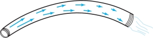
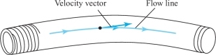
The flow of water through a pipe is said to be steady if, at each point inside the pipe, the velocity of the fluid passing through that point does not change with time. (Note that this is quite different from saying that the water in the pipe is not moving.) Attaching to each point the fluid velocity at that point, we obtain the velocity field \({\bf V}\) of the fluid (see Figure 4.20). Notice that the length of the arrows (the speed), as well as the direction of flow, may change from point to point.
example 2
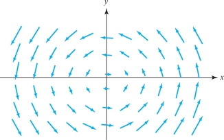
Some forms of rotary motion (such as the motion of particles on a turntable) can be described by the vector field \[ {\bf V}(x,y)=-y{\bf i}+x{\bf j}. \]
See Figure 4.21, in which we have shown instead of \({\bf V}\) the shorter vector field \(\frac{1}{4}{\bf V}\) so that the arrows do not overlap. This is a common convention in drawing pictures of vector fields.
example 3
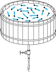
In the plane, \({\mathbb R}^2\), let the vector field \(x\) be defined by \[ {\bf V}(x,y)=\frac{y{\bf i}}{x^2+y^2}-\frac{x{\bf j}}{x^2+y^2}=\bigg(\frac{y}{x^2+y^2},-\frac{x}{x^2+y^2}\bigg) \] (except at the origin, where \({\bf V}\) is not defined). This vector field is a good approximation to the planar part of the velocity of water flowing toward a hole in the bottom of a tub (Figure 4.22). Notice that the velocity becomes larger as you approach the hole.
Gradient Vector Fields
238
In Section 2.6 we introduced the gradient of a function by \[ \nabla f(x,y,z)=\frac{\partial f}{\partial x}(x,y,z){\bf i}+\frac{\partial f}{\partial y}(x,y,z){\bf j}+\frac{\partial f}{\partial z}(x,y,z){\bf k}. \]
Now we want to think of this as an example of a vector field—it assigns a vector to each point (\(x, y, z\)). As such, we refer to \(\nabla f\) as a gradient vector field. Gradient fields come up in a variety of situations, as the next two examples show.
example 4
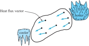
A piece of material is heated on one side and cooled on another. The temperature at each point within the body is described at a given moment by a scalar field \(T(x,y,z)\). The flow of heat may be marked by a field of arrows indicating the direction and magnitude of the flow (Figure 4.23). This energy or heat flux vector field is given by \({\bf J}=-k {\nabla} T\), where \(k>0\) is a constant called the conductivity and \({\nabla} T\) is the gradient of the real-valued function \(T\). Level sets of \(T\) are called isotherms. Note that the heat flows from hot regions toward cold ones, since \(-{\nabla} T\) points in the direction of decreasing \(T\).
example 5
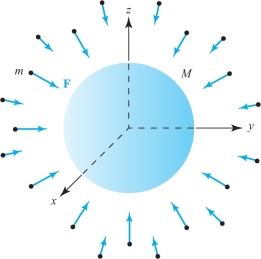
The force of attraction of the earth on a mass \(m\) can be described by a vector field called the gravitational force field. Place the origin of a coordinate system at the center of the earth (assumed spherical). According to Newton’s law of gravity, this field is given by \[ {\bf F}=-\frac{m{\it MG}}{r^3}{\bf r}, \] where \({\bf r}(x,y,z)=(x,y,z)\), and \(r=\|{\bf r}\|\) (see Figure 4.24). The domain of this vector field consists of those \(\bf r\) for which \(\|{\bf r}\|\) is greater than the radius of the earth. As we saw in Example 6, Section 2.6, \({\bf F}\) is a gradient field, \({\bf F}=-{\nabla} V\), where \[ V=-\frac{m{\it MG}}{r} \] is the gravitational potential. Note again that \({\bf F}\) points in the direction of decreasing \(V\). Writing \({\bf F}\) in terms of components, we see that \[ {\bf F}(x,y,z)=\bigg(\frac{-m{\it MG}}{r^3}x,\frac{-m{\it MG}}{r^3}y, \frac{-m{\it MG}}{r^3}z\bigg). \]
239
example 6
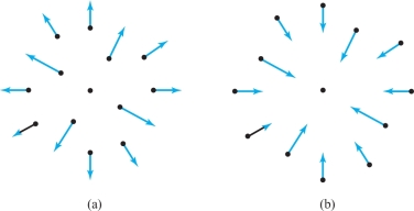
According to Coulomb’s law, the force acting on a charge \(e\) at position \({\bf r}\) due to a charge \(Q\) at the origin is \[ {\bf F}=\frac{\varepsilon Q e}{r^3}{\bf r}=-{\nabla} V, \] where \(V=\varepsilon Q e /r\) and \(\varepsilon\) is a constant that depends on the units used. For \(Qe >0\) (like charges) the force is repulsive [Figure 4.25], and for \(Qe < 0\) (unlike charges) the force is attractive [Figure 4.25]. Because the potential \(V\) is constant on the level surfaces of \(V\), they are called equipotential surfaces. Note that the force field is orthogonal to the equipotential surfaces (the force field is radial and the equipotential surfaces are concentric spheres).
The next example shows that not every vector field is a gradient.
example 7
Show that the vector field \({\bf V}\) on \({\mathbb R}^2\) defined by \({\bf V}(x,y)=y{\bf i}-x{\bf j}\) is not a gradient vector field; that is, there is no \(C^1\) function \(f\) such that \[ {\bf V}(x,y)= \nabla \! f(x,y)=\frac{\partial f}{\partial x}{\bf i}+ \frac{\partial f}{\partial y}{\bf j}. \]
solution Suppose that such an \(f\) exists. Then \(\partial f/\partial x=y\) and \(\partial f/\partial y=-x\). Because these are \(C^1\) functions, \(f\) itself must have continuous first- and second-order partial derivatives. But, \({\partial^2\! f}/\partial x\,\partial y =\,{-}1\), and \(\partial^2\! f/\partial y\,\partial x =1\), which violates the equality of mixed partials. Thus, \({\bf V}\) cannot be a gradient vector field.
Conservation of Energy and Escaping the Earth’s Gravitational Field
240
Consider a particle of mass \(m\) moving in a force field \({\bf F}\) that is a potential field. That is, assume \({\bf F}\,{=}\,{-}\nabla V\) for a real-valued function \(V\), and that the particle moves according to \({\bf F}\,{=}\,m{\bf a}\). Thus, if the path is \({\bf r}(t)\), then \begin{equation} m\ddot{\bf r}(t) = {-}\nabla V({\bf r}(t)). \end{equation}
A basic fact about such motion is the conservation of energy. The energy \(E\) of the particle is defined to be the sum of the kinetic and potential energies, defined as \begin{equation} E=\frac{1}{2}m\|\dot{\bf r}(t)\|^2+V({\bf r}(t)). \end{equation}
The principle of conservation of energy states that if Newton’s second law holds, then \(E\) is independent of time; that is, \({\it dE}{/}{\it dt}\,{=}\,0\). The proof of this fact is a simple calculation; we use equation (2), the chain rule, and equation (1): \begin{eqnarray*} \frac{{\it dE}}{{\it dt}} &=& m\dot{\bf r}\,{\cdot}\,\ddot{\bf r}+(\nabla V)\,{\cdot}\,\dot{\bf r}\\[4pt] &=&\dot{\bf r}\,{\cdot}\,(-\nabla V+\nabla V)=0. \end{eqnarray*}
Escape Velocity
As an application of conservation of energy, we compute the velocity required for a rocket to escape the earth's gravitational influence. Assume the rocket has mass \(m\) and is at a distance \(R_{0}\) from the center of the earth (or another planet) when its escape velocity \(v_{e}\) has been reached, and that it will coast thereafter. The energy at this time is \begin{equation} E_0=\frac{1}{2}mv^2_e - \frac{m{\it MG}}{R_0}. \end{equation}
By conservation of energy, \(E_{0}\) will equal the energy at a later time, which we write as \begin{equation} E_0=E=\frac{1}{2}mv^2 - \frac{m{\it MG}}{R}, \end{equation} where \(v\) is the velocity and \(R\) is the distance from the center of the earth (or the other planet). What we mean by the term escape velocity is that \(v_{e}\) is chosen such that the rocket gets to great distances, at which time it is barely moving. That is, \(v\) is close to zero and \(R\) is very large. Thus, from equation (4), we see that \(E = 0\) and hence \(E_{0} = 0\); solving \(E_{0} = 0\) for \(v_{e}\) using equation (3) gives: \[ v_e = \sqrt{\frac{2{\it MG}}{R_0}}. \]
241
Now \({\it GM}/R^{2}_{0}\) is exactly \(g\), the acceleration due to gravity at the distance \(R_{0}\) from the center of the planet. Thus, we can write: \[ v_e=\sqrt{2gR_0}. \]
For the earth, if the escape velocity were to be achieved at the surface of the earth (of course, this is a bit unrealistic), this would give \[ v_e=\sqrt{2\,{\cdot}\,9.8 \ {\rm m\hbox{/}s}^2{\cdot}\,\hbox{6,371,000} \ {\rm m}}=\hbox{11,127} \ {\rm m\hbox{/}s}. \]
However, this is a good approximation to the velocity that a satellite in low earth orbit needs in order to escape the earth’s gravitational field.
Flow Lines
An important concept related to general (not necessarily gradient) vector fields is that of a flow line, defined as follows.
Flow Lines
If \({\bf F}\) is a vector field, a flow line for \({\bf F}\) is a path \({\bf c}(t)\) such that \[ {\bf c}'(t)={\bf F}({\bf c}(t)). \]
In the context of Example 1, a flow line is the path followed by a small particle suspended in the fluid (Figure 4.26). Flow lines are also appropriately called streamlines or integral curves.
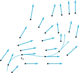
Geometrically, a flow line for a given vector filed \({\bf F}\) is a curve that threads its way through the domain of the vector field in such a way that the tangent vector of the curve coincides with the vector field, as in Figure 4.27.
242
A flow line may be viewed as a solution of a system of differential equations. Indeed, we can write the definition \({\bf c}'(t)={\bf F}({\bf c}(t))\) as \begin{eqnarray*} x'(t) &=& P(x(t),y(t),z(t)),\\[3pt] y'(t) &=& Q(x(t),y(t),z(t)),\\[3pt] z'(t) &=& R(x(t),y(t),z(t)), \end{eqnarray*} where \({\bf c}(t)=x(t){\bf i}+y(t){\bf j}+z(t){\bf k}\), and where \[ {\bf F}=P{\bf i}+Q{\bf j}+R{\bf k}. \]
You probably learned about such systems in courses on differential equations, but we are not presuming such a course has been taken.
example 8
Show that the path \({\bf c}(t)=(\cos t,\,\sin t)\) is a flow line of the vector field \({\bf F}(x,y)=-y{\bf i}+x{\bf j}\). Can you find others?
solution We must verify that \({\bf c}'(t)={\bf F}({\bf c}(t))\). The left side is \(({-}{\sin t}){\bf i}+(\cos t){\bf j}\), while the right side is \({\bf F}(\cos t,\,\sin t)=({-}{\sin t}){\bf i}+(\cos t){\bf j}\), so we have a flow line. As suggested by Figure 4.21, the other flow lines are also circles. They have the form \[ {\bf c}(t)=(r\,\cos\, (t-t_0),r\,\sin\, (t-t_0)) \] for constants \(r\) and \(t_0\).
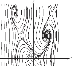
In many cases, explicit formulas for flow lines are not available, so we must resort to numerical methods. Figure 4.28 shows some output from a program that computes flow lines numerically and plots them on the screen.
Historical Note
The Field Concept
The concept of a “field,” such as a vector field, has had an enormous impact on the development of conceptual frameworks for physics and engineering. It is truly one of the great breakthrough ideas in the history of human thought. It is the notion that allows us to describe, in a systematic way, influences on objects and between objects that are spatially separated.
243
The idea of a field began with Newton’s concept of the gravitational field. In this case, the gravitational field describes the attractive influence of a group of bodies on each other. Similarly, the electric field produced by a charged object or group of objects creates, according to Coulomb’s law, a force on another charged object. Using vector fields to describe these sorts of forces has led to a deeper understanding of attractive and repulsive forces in nature.
However, it was the monumental discovery of the Maxwell field equations, which describe the propagation of electromagnetic energy, that cemented the concept of “field” in scientific thought. This example is particularly interesting because these fields can propagate. The contrast between the electromagnetic field that can propagate and the gravitational field that involves instantaneous action at a distance has caused great interest among philosophers of science.
Einstein’s idea is that gravitation can be described in terms of the metric properties of space–time and that in this theory the associated field can also propagate, just like the electromagnetic field, thus providing profound philosophical evidence that Einstein’s version of gravity may be correct. These ideas have also led to modern efforts to detect gravitational waves. For a further discussion of Einstein’s work, see Section 7.7.
The idea of a field is also used in engineering to describe elastic systems and interesting microstructural properties of materials. In modern theoretical physics, the field concept is used to describe elementary particles and is central to attempts by modern theoretical physicists to unify gravity with the quantum mechanical physics of elementary particles. It is impossible to imagine a modern theoretical framework that does not incorporate some sort of field concept as a central ingredient.