5.3 The Double Integral Over a Rectangle

We are ready to give a rigorous definition of the double integral as the limit of a sequence of sums. This will then be used to define the volume of the region under the graph of a function \(f(x, y)\). We shall not require that \(f(x,y) \geq 0\); but if \(f(x, y)\) assumes negative values, we shall interpret the integral as a signed volume, just as for the area under the graph of a function of one variable. In addition, we shall discuss some of the fundamental algebraic properties of the double integral and prove Fubini’s theorem, which states that the double integral can be calculated as an iterated integral. To begin, let us establish some notation for partitions and sums.

Definition of the Integral

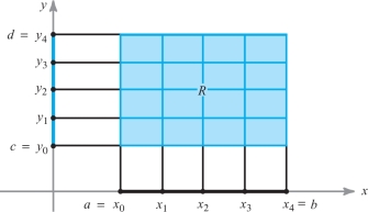
Consider a closed rectangle \(R\subset {\mathbb R}^2\); that is, \(R\) is a Cartesian product of two intervals: \(R=[a,b]\times [c,d]\). By a regular partition of \(R\) of order \(n\) we mean the two ordered collections of \(n+1\) equally spaced points \(\{x_j\}^n_{j=0}\) and \(\{y_k\}^n_{k=0}\); that is, the points satisfying \[ a=x_0<x_1<\cdots<x_n=b, c=y_0<y_1<\cdots<y_n=d \] and \[ x_{j+1}-x_j=\frac{b-a}{n}, y_{k+1}-y_k=\frac{d-c}{n} \] (see Figure 5.14).

A function \(f(x,y)\) is said to be bounded if there is a number \(M>0\) such that \(-M\leq f(x,y)\leq M\) for all \((x, y)\) in the domain of \(f\). A continuous function on a closed rectangle is always bounded, but, for example, \(f(x,y)=1/x\) on \((0,1]\times [0,1]\) is continuous but is not bounded, because \(1/x\) becomes arbitrarily large for \(x\) near 0. The rectangle \((0,1]\times [0,1]\) is not closed, because the endpoint \(0\) is missing in the first factor.

Let \(R_{jk}\) be the rectangle \([x_j,x_{j+1}]\times [y_k,y_{k+1}]\), and let \({\bf c}_{jk}\) be any point in \(R_{jk}\). Suppose \(f\colon R \to {\mathbb R}\) is a bounded real-valued function. Form the sum \begin{equation*} S_n=\sum_{j,k=0}^{n-1}f({\bf c}_{\it jk})\ \Delta x\ \Delta y=\sum_{j,k=0}^{n-1} f({\bf c}_{\it jk})\ \Delta A,\tag{1} \end{equation*} where \[ \Delta x=x_{j+1}-x_j=\frac{b-a}{n}, \Delta y=y_{k+1} -y_k=\frac{d-c}{n}, \] and \[ \Delta A=\Delta x\ \Delta y . \]

This sum is taken over all \(j\)’s and \(k\)’s from 0 to \(n -1\), and so there are \(n^2\) terms. A sum of this type is called a Riemann sum for \(f\).

Thus, we can rewrite integrability in the following way: \[ \mathop{\rm limit}_{n \to \infty} \sum_{j,k=0}^{n-1}f({\bf c}_{\it jk})\ \Delta x\ \Delta y= \intop\!\!\!\intop\nolimits_{R} f{\it dx}\,{\it dy} \] for any choice of \({\bf c}_{\it jk}\in R_{\it jk}\).

Properties of the Integral

The proof of the following basic theorem is presented in the Internet supplement for Chapter 5.

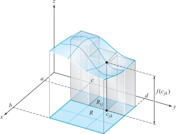
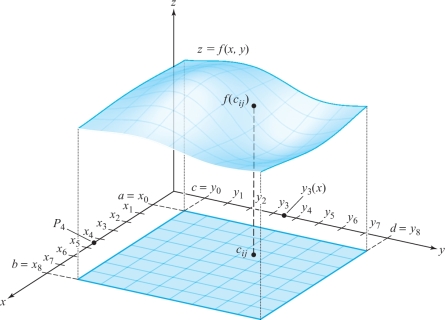
If \(f(x,y)\geq 0\), the existence of \(\mathop{\rm limit}_{n\to \infty} S_n\) has a straightforward geometric meaning. Consider the graph of \(z=f(x,y)\) as the top of a solid whose base is the rectangle \(R\). If we take each \({\bf c}_{\it jk}\) to be a point where \(f(x, y)\) has its minimum valuefootnote # on \(R_{\it jk}\), then \(f({\bf c}_{\it jk})\, \Delta x\, \Delta y\) represents the volume of a rectangular box with base \(R_{\it jk}\). The sum \(\sum_{j, k=0}^{n-1}f({\bf c}_{\it jk})\, \Delta x\, \Delta y\) equals the volume of an inscribed solid, part of which is shown in Figure 5.15.

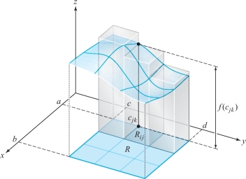
Similarly, if \({\bf c}_{\it jk}\) is a point where \(f(x,y)\) has its maximum on \(R_{\it jk}\), then the sum \(\sum_{j,k=0}^{n-1}f({\bf c}_{\it jk})\, \Delta x\, \Delta y\) is equal to the volume of a circumscribed solid (see Figure 5.16).

Therefore, if \(\mathop{\rm limit}_{n\to \infty}S_n\) exists and is independent of \({\bf c}_{\it jk}\in R_{\it jk}\), it follows that the volumes of the inscribed and circumscribed solids approach the same limit as \(n\to \infty\). It is therefore reasonable to call this limit the exact volume of the solid under the graph of \(f\). Thus, the method of Riemann sums supports the concepts introduced on an intuitive basis in Section 5.2.

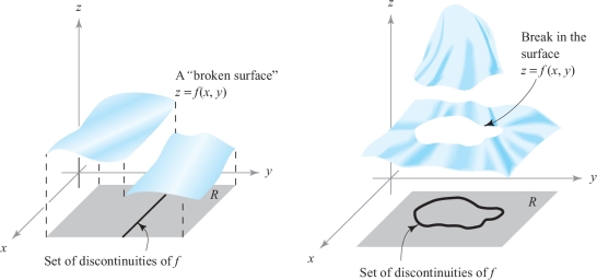
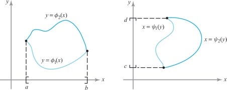
There is a theorem guaranteeing the existence of the integral of certain discontinuous functions as well. We shall need this result in the next section in order to discuss the integrals of functions over regions more general than rectangles. We shall be specifically interested in functions whose discontinuities lie on curves in the \(xy\) plane. Figure 5.17 shows two functions defined on a rectangle \(R\) whose discontinuities lie along curves. In other words, \(f\) is continuous at each point that is in \(R\), but not necessarily on the curve.

Useful curves are graphs of functions such as \(y=\phi(x), a\leq x\leq b\), or \(x=\psi(y), c\leq y\leq d\), or finite unions of such graphs. Some examples are shown in Figure 5.18.

The next theorem provides an important criterion for determining whether a function is integrable. The proof is discussed in the Internet supplement.

Using Theorem 2 and the remarks preceding it, we see that the functions sketched in Figure 5.17 are integrable over \(R\), because these functions are bounded and continuous except on graphs of continuous functions.

From the definition of the integral as a limit of sums and the limit theorems, we can deduce some fundamental properties of the integral \({\intop\!\!\!\intop}_Rf(x,y)\, {\it dA}\); these properties are essentially the same as for the integral of a real-valued function of a single variable.

Let \(f\) and \(g\) be integrable functions on the rectangle \(R\), and let \(c\) be a constant. Then \(f + g\) and \(cf\) are integrable, and

• (i) Linearity \[ \intop\!\!\!\intop\nolimits_{R}\, [f(x,y)+g(x,y)]\, {\it dA}= \intop\!\!\!\intop\nolimits_{R} \, f(x,y)\, {\it dA}+ \intop\!\!\!\intop\nolimits_{R} \, g(x,y)\, {\it dA}. \]
• (ii) Homogeneity \[ \intop\!\!\!\intop\nolimits_{R}\, cf(x,y)\, {\it dA}=c \intop\!\!\!\intop\nolimits_{R}\, f(x,y)\, {\it dA}. \]
• (iii) Monotonicity If \(f(x,y)\geq g(x,y)\), then \[ \intop\!\!\!\intop\nolimits_{R}\, f(x,y)\, {\it dA}\geq \intop\!\!\!\intop\nolimits_{R}\, g(x,y)\, {\it dA}. \]
• (iv) Additivity If \(R_i, i=1,\ldots, m\), are pairwise disjoint rectangles such that \(f\) is bounded and integrable over each \(R_i\) and if \(Q=R_1\cup R_2\cup\cdots \cup R_m\) is a rectangle, then \(f\colon Q\to {\mathbb R}\) is integrable over \(Q\) and \[ \intop\!\!\!\intop\nolimits_{Q}f(x,y)\, {\it dA}= \sum_{i=1}^m\intop\!\!\!\intop\nolimits_{R_i}f(x,y)\, {\it dA}. \]

Properties (i) and (ii) are a consequence of the definition of the integral as a limit of a sum and the following facts for convergent sequences \(\{S_n\}\) and \(\{T_n\}\), which are proved as with the limit theorems in Chapter 2: \begin{eqnarray*} \mathop{\rm limit}_{n\to \infty} \ (T_n+S_n)&=&\mathop{\rm limit}_{n\to \infty} T_n +\mathop{\rm limit}_{n\to \infty} S_n\\[3pt] \mathop{\rm limit}_{n\to \infty}\ (cS_n)&=&c\mathop{\rm limit}_{n\to \infty} S_n. \end{eqnarray*}

To demonstrate monotonicity, we first observe that if \(h(x,y)\geq 0\) and \(\{S_n\}\) is a sequence of Riemann sums that converges to \({\intop\!\!\!\intop}_R h(x,y)\, {\it dA}\), then \(S_n\geq 0\) for all \(n\), so that \({\intop\!\!\!\intop}_R h(x,y)\, {\it dA}= {\rm limit}_{n\to \infty} S_n \geq 0\). If \(f(x,y)\geq g(x,y)\) for all \((x,y)\in R\), then \((f-g)(x,y)\geq 0\) for all \((x, y)\), and, using properties (i) and (ii), we have \[ \intop\!\!\!\intop\nolimits_{R}\, f(x,y)\, {\it dA}- \intop\!\!\!\intop\nolimits_{R}\, g(x,y)\, {\it dA}= \intop\!\!\!\intop\nolimits_{R}\, [f(x,y)-g(x,y)]\, {\it dA}\geq 0. \]

This proves property (iii). The proof of property (iv) is more technical, and a special case is proved in the Internet supplement. It should be intuitively obvious.

Another important result is the inequality \begin{equation*} \bigg|\intop\!\!\!\intop\nolimits_{R}\, f\,{\it dA}\bigg|\leq \intop\!\!\!\intop\nolimits_{R}\, |f|\, {\it dA}.\tag{2} \end{equation*}

To see why formula (2) is true, note that, by the definition of absolute value, \[ -|f|\leq f \leq |f|; \] therefore, from the monotonicity and homogeneity of integration (with \(c = -1\)), \[ - \intop\!\!\!\intop\nolimits_{R}\, |f|\,{\it dA}\leq \intop\!\!\!\intop\nolimits_{R}\, f\,{\it dA}\leq \intop\!\!\!\intop\nolimits_{R}\, |f|\,{\it dA}, \] which is equivalent to formula (2).

Fubini’s Theorem

Although we have noted the integrability of a variety of functions, we have not yet established rigorously a general method of computing integrals. In the case of one variable, we avoid computing \(\int_a^b f(x)\, {\it dx}\) from its definition as a limit of a sum by using the fundamental theorem of integral calculus. This important theorem tells us that if f is continuous, then \[ \int_a^bf(x)\, {\it dx} =F(b)-F(a), \] where \(F\) is an antiderivative of \(f\); that is, \(F'=f\).

This technique will not work as stated for functions \(f(x,y)\) of two variables. However, as we indicate in Section 5.2, we can often reduce a double integral over a rectangle to iterated single integrals; the fundamental theorem then applies to each of these single integrals. Fubini’s theorem, which was mentioned in the last section, establishes this reduction to iterated integrals rigorously, by using Riemann sums. As we saw in Section 5.2, the reduction, \[ \intop\!\!\!\intop\nolimits_{R} \, f(x,y)\, {\it dA}=\int_a^b \bigg[ \int_c^d\, f(x,y)\, {\it dy} \bigg]\, {\it dx} = \int_c^d \bigg[ \int_a^bf(x,y)\, {\it dx} \bigg]\, {\it dy}, \] is a consequence of Cavalieri’s principle, at least if \(f(x,y)\geq 0\). In terms of Riemann sums, it corresponds to the following equality: \[ \sum_{j,k=0}^{n-1}f({\bf c}_{\it jk})\, \Delta x\, \Delta y= \sum_{j=0}^{n-1}\left(\sum_{k=0}^{n-1}f({\bf c}_{\it jk})\, \Delta y\right)\Delta x =\sum_{k=0}^{n-1}\left(\sum_{j=0}^{n-1}f({\bf c}_{\it jk})\, \Delta x\right)\Delta y, \] which may be proved more generally as follows: Let \([a_{\it jk}]\) be an \(n\times n\) matrix, where \(0\leq j\leq n-1\) and \(0\leq k\leq n-1\). Let \(\sum_{j,k=0}^{n-1} a_{\it jk}\) be the sum of the \(n^2\) matrix entries. Then \begin{equation*} \sum_{j,k=0}^{n-1}a_{\it jk}=\sum_{j=0}^{n-1}\left(\sum_{k=0}^{n-1}a_{\it jk}\right)=\sum_{k=0}^{n-1} \left(\sum_{j=0}^{n-1}a_{\it jk}\right).\tag{3} \end{equation*}

In the first equality, the right-hand side represents summing the matrix entries first by rows and then adding the results:

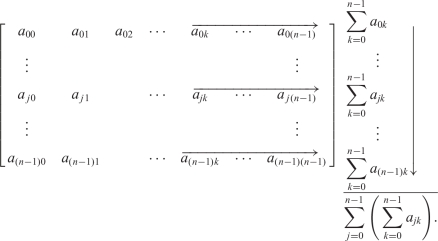
Clearly, this is equal to \(\sum_{j,k=0}^{n-1}a_{\it jk}\); that is, the sum of all the \(a_{\it jk}\). Similarly, the sum \(\sum_{k=0}^{n-1}\) \(\big(\sum_{j=0}^{n-1} a_{\it jk}\big)\) represents a summing of the matrix entries by columns. This establishes equation (3) and makes the reduction to iterated integrals quite plausible if we remember that integrals can be approximated by the corresponding Riemann sums. The actual proof of Fubini’s theorem exploits this idea.

Fubini’s theorem can be generalized to the case where \(f\) is not necessarily continuous. Although we shall not present a proof, we state here this more general version.

The assumptions made for this version of Fubini’s theorem are more complicated than those we made in Theorem 3. They are necessary because if \(f\) is not continuous everywhere, for example, there is no guarantee that \(\int_c^df(x,y)\, {\it dy}\) will exist for each \(x\).

We have seen that when \(f(x,y)\geq 0\) on \(R=[a,b]\times [c,d]\), the integral \(\intop\!\!\!\intop\nolimits_{R}f(x,y) \,{\it dA}\) can be interpreted as a volume. If the function also takes on negative values, then the double integral can be thought of as the sum of all volumes lying between the surface \(z = f(x, y)\) and the plane \(z = 0\), bounded by the planes \(x=a, x=b, y=c\), and \(y=d\); here the volumes above \(z=0\) are counted as positive and those below as negative. However, Fubini’s theorem as stated remains valid in the case where \(f(x, y)\) is negative or changes sign on \(R\); that is, there is no restriction on the sign of \(f\) in the hypotheses of the theorem.