11.7 Polar coordinates
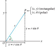
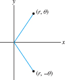
In polar coordinates, we label a point \(P\) by coordinates \((r,\theta)\), where \(r\) is the distance to the origin \(O\) and \(\theta\) is the angle between \(\overline{OP}\) and the positive \(x\)-axis (Figure 11.38). By convention, an angle is positive if the corresponding rotation is counterclockwise. We call \(r\) the radial coordinate and \(\theta\) the angular coordinate.
Note
Polar coordinates are appropriate when distance from the origin or angle plays a role. For example, the gravitational force exerted on a planet by the sun depends only on the distance \(r\) from the sun and is conveniently described in polar coordinates.
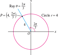
The point \(P\) in Figure 11.39 has polar coordinates \((r, \theta) =\big(4,\frac{2\pi}3\big)\). It is located at distance \(r= 4\) from the origin (so it lies on the circle of radius 4), and it lies on the ray of angle \(\theta=\frac{2\pi}{3}\).
Figure 11.40 shows the two families of grid lines in polar coordinates: \[ \begin{array}\\ \hbox{Circle centered at \(O\)} & \longleftrightarrow & r &{}={}& \hbox{constant}\\ \hbox{Ray starting at \(O\)} & \longleftrightarrow &\theta &=& \hbox{constant} \end{array} \]
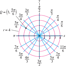
Every point in the plane other than the origin lies at the intersection of the two grid lines and these two grid lines determine its polar coordinates. For example, point \(Q\) in Figure 3 lies on the circle \(r=3\) and the ray \(\theta = \frac{5\pi}6\), so \(Q=\big(3,\frac{5\pi}6\big)\) in polar coordinates.
Figure 11.38 shows that polar and rectangular coordinates are related by the equations \(x=r\cos\theta\) and \(y=r\sin \theta\). On the other hand, \(r^2=x^2+y^2\) by the distance formula, and \(\tan\theta={y}/{x}\) if \(x \neq 0\). This yields the conversion formulas:
| Polar to Rectangular | Rectangular to Polar |
| \(x=r\cos\theta\) | \(r=\sqrt{x^2+y^2}\) |
| \(y = r\sin\theta\) | \(\tan\theta=\frac{y}{x}\quad (x\neq 0)\) |
627
EXAMPLE 1 From Polar to Rectangular Coordinates
Find the rectangular coordinates of point \(Q\) in Figure 11.40.
Solution The point \(Q= (r,\theta) = \big(3,\frac{5\pi}6\big)\) has rectangular coordinates: \begin{align*} x &= r\cos\theta = 3\cos\left(\frac{5\pi}6\right) =3\left(-\frac{\sqrt{3}}2\right) = -\frac{3\sqrt{3}}2\\ y &= r\sin\theta =3\sin\left(\frac{5\pi}6\right) =3\left(\frac{1}2\right) = \frac32 \end{align*}
EXAMPLE 2 From Rectangular to Polar Coordinates
Find the polar coordinates of point \(P\) in Figure 11.41.
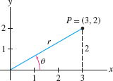
Solution Since \(P=(x,y)=(3,2)\), \begin{align*} r&=\sqrt{x^2+y^2}=\sqrt{3^2+2^2}=\sqrt{13}\approx 3.6\\ \tan\theta &= \frac{y}{x} = \frac23 \end{align*} and because \(P\) lies in the first quadrant, \begin{align*} \theta &= \tan^{-1} \frac{y}x = \tan^{-1} \frac23 \approx 0.588 \end{align*} Thus, \(P\) has polar coordinates \((r,\theta) \approx (3.6,0.588)\).
Definition
By definition, \[ -\frac{\pi}2<\tan^{-1} x < \frac{\pi}2 \] If \(r>0\), a coordinate \(\theta\) of \(P=(x,y)\) is \[ \theta = \begin{cases} \tan^{-1}\frac{y}x & \text{ if \(x > 0\)} \\ \tan^{-1}\frac{y}x +\pi & \text{ if \(x<0\)}\\ \pm \frac{\pi}{2}& \text{ if \(x = 0\)} \end{cases} \]}
A few remarks are in order before proceeding:
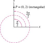
- The angular coordinate is not unique because \((r,\theta)\) and \((r,\theta+2\pi n)\) label the same point for any integer \(n\). For instance, point \(P\) in Figure 11.42 has radial coordinate \(r=2\), but its angular coordinate can be any one of \(\frac{\pi}2\), \(\frac{5\pi}2,\ldots\) or \(-\frac{3\pi}2\), \(-\frac{7\pi}2, \ldots.\)
- The origin \(O\) has no well-defined angular coordinate, so we assign to \(O\) the polar coordinates \((0,\theta)\) for any angle \(\theta\).
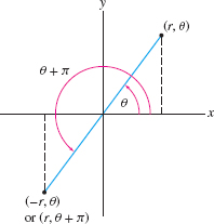
- By convention, we allow negative radial coordinates. By definition, \((-r,\theta)\) is the reflection of \((r,\theta)\) through the origin (Figure 11.43). With this convention, \((-r,\theta)\) and \((r,\theta+\pi)\) represent the same point.
- We may specify unique polar coordinates for points other than the origin by placing restrictions on \(r\) and \(\theta\). We commonly choose \(r>0\) and \(0\le \theta < 2\pi\).
628
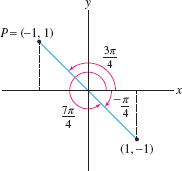
When determining the angular coordinate of a point \(P=(x,y)\), remember that there are two angles between \(0\) and \(2\pi\) satisfying \(\tan\theta= {y}/x\). You must choose \(\theta\) so that \((r,\theta)\) lies in the quadrant containing \(P\) and in the opposite quadrant (Figure 11.44).
EXAMPLE 3 Choosing \(\theta\) Correctly
Find two polar representations of \(P = (-1,1)\), one with \(r>0\) and one with \(r<0\).
Solution The point \(P=(x,y) = (-1,1)\) has polar coordinates \((r,\theta)\), where \[ r=\sqrt{(-1)^2+1^2}=\sqrt 2,\qquad \tan\theta=\tan\frac{y}{x}=-1 \] However, \(\theta\) is not given by \[ \tan^{-1}\frac{y}x = \tan^{-1}\left(\frac1{-1}\right) = -\frac{\pi}4 \] because \(\theta = -\frac{\pi}4\) this would place \(P\) in the fourth quadrant (Figure 11.44). Since \(P\) is in the second quadrant, the correct angle is \[ \theta =\tan^{-1}\frac{y}x +\pi = -\frac{\pi}4 + \pi = \frac{3\pi}4 \] If we wish to use the negative radial coordinate \(r= -\sqrt 2\), then the angle becomes \(\theta= -\frac{\pi}4\) or \(\frac{7\pi}4\). Thus, \[ P = \left(\sqrt 2,\frac{3\pi}4\right)\qquad \textrm{or} \qquad \left(-\sqrt 2,\frac{7\pi}4\right) \]
A curve is described in polar coordinates by an equation involving \(r\) and \(\theta\), which we call a polar equation. By convention, we allow solutions with \(r<0\).
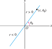
A line through the origin \(O\) has the simple equation \(\theta=\theta_0\), where \(\theta_0\) is the angle between the line and the \(x\)-axis (Figure 11.45). Indeed, the points with \(\theta=\theta_0\) are \((r,\theta_0)\), where \(r\) is arbitrary (positive, negative, or zero).
EXAMPLE 4 Line Through the Origin
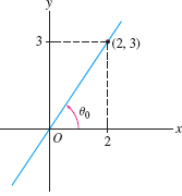
Find the polar equation of the line through the origin of slope \(\frac32\) (Figure 11.46).
Solution A line of slope \(m\) makes an angle \(\theta_0\) with the \(x\)-axis, where \(m=\tan\theta_0\). In our case, \(\theta_0 = \tan^{-1}\frac32 \approx 0.98\). The equation of the line is \(\theta= \tan^{-1} \frac32\) or \(\theta \approx 0.98\).
To describe lines that do not pass through the origin, we note that any such line has a unique point \(P_0\) that is closest to the origin. The next example shows how to write down the polar equation of the line in terms of \(P_0\) (Figure 11.47).
629
EXAMPLE 5 Line Not Passing Through \(O\)
Show that \begin{equation} \boxed{\bbox[#fef7e5,5pt]{r=d\sec(\theta-\alpha)}}\tag{1} \end{equation} is the polar equation of the line \(L\) whose point closest to the origin is \(P_0 = (d,\alpha)\).
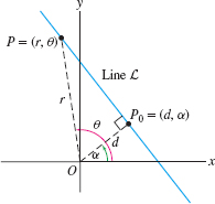
Solution The point \(P_0\) is obtained by dropping a perpendicular from the origin to \(L\) (Figure 11.48), and if \(P = (r,\theta)\) is any point on \(L\) other than \(P_0\), then \(\triangle \textit{OPP}_0\) is a right triangle. Therefore, \({d}/{r} = \cos(\theta - \alpha)\), or \(r = d\sec(\theta - \alpha)\), as claimed.
EXAMPLE 6
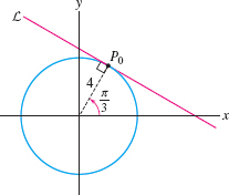
Find the polar equation of the line \(L\) tangent to the circle \(r=4\) at the point with polar coordinates \(P_0=\big(4,\frac{\pi}3\big)\).
Solution The point on \(L\) closest to the origin is \(P_0\) itself (Figure 11.48). Therefore, we take \((d,\alpha)=\big(4,\frac{\pi}3\big)\) in Eq. (1) to obtain the equation \(r=4\sec\big(\theta-\frac{\pi}3\big)\).
Often, it is hard to guess the shape of a graph of a polar equation. In some cases, it is helpful rewrite the equation in rectangular coordinates.
EXAMPLE 7 Converting to Rectangular Coordinates
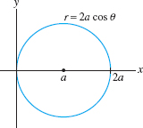
Identify the curve with polar equation \(r=2a\cos\theta\) (\(a\) a constant).
Solution Multiply the equation by \(r\) to obtain \(r^2=2ar\cos\theta\). Because \(r^2=x^2+y^2\) and \(x=r\cos\theta\), this equation becomes \[ x^2+y^2 = 2ax\qquad\textrm{or}\qquad x^2-2ax+y^2= 0 \] Then complete the square to obtain \((x-a)^2+y^2=a^2\). This is the equation of the circle of radius \(a\) and center \((a,0)\) (Figure 11.49).
A similar calculation shows that the circle \(x^2 + (y-a)^2 = a^2\) of radius \(a\) and center \((0,a)\) has polar equation \(r=2a\sin\theta\). In the next example, we make use of symmetry. Note that the points \((r,\theta)\) and \((r,-\theta)\) are symmetric with respect to the \(x\)-axis (Figure 11.50).
EXAMPLE 8 Symmetry About the \(x\)-Axis
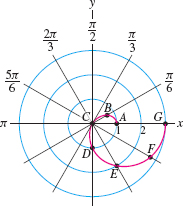
Sketch the limaçon curve \newline \(r = 2\cos\theta-1\).
Solution Since \(\cos\theta\) is periodic, it suffices to plot points for \(-\pi\le \theta\le \pi\).
Step 1. Plot points
To get started, we plot points \(A\)–\(G\) on a grid and join them by a smooth curve (Figure 11.51).
630
| \(A\) | \(B\) | \(C\) | \(D\) | \(E\) | \(F\) | \(G\) | |
| \(\theta\) | 0 | \(\frac{\pi}6\) | \(\frac{\pi}3\) | \(\frac{\pi}2\) | \(\frac{2\pi}3\) | \(\frac{5\pi}6\) | \(\pi\) |
| \(r= 2 \cos \theta -1\) | 1 | 0.73 | 0 | \(-1\) | \(-2\) | \(-2.73\) | \(-3\) |
Step 2. Analyze \(r\) as a function of \(\theta\)
For a better understanding, it is helpful to graph \(r\) as a function of \(\theta\) in rectangular coordinates. Figure 11.52 shows that
| As \(\theta\) varies from 0 to \(\frac{\pi}3\), | \(r\) varies from 1 to 0. |
| As \(\theta\) varies from \(\frac{\pi}3\) to \(\pi\), | \(r\) is negative and varies from 0 to \(-3\). |
We conclude:
- The graph begins at point \(A\) in Figure 11.52 and moves in toward the origin as \(\theta\) varies from \(0\) to \(\frac{\pi}3\).
- Since \(r\) is negative for \(\frac{\pi}3\le\theta\le \pi\), the curve continues into the third and fourth quadrants (rather than into the first and second quadrants), moving toward the point \(G = (-3,\pi)\) in Figure 11.52.
Step 3. Use symmetry
Since \(r(\theta)=r(-\theta)\), the curve is symmetric with respect to the \(x\)-axis. So the part of the curve with \(-\pi\le\theta\le 0\) is obtained by reflection through the \(x\)-axis as in Figure 11.52.
