GRAPHICAL INSIGHT

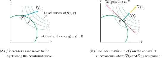
Imagine standing at point \(Q\) in Figure 14.71. We want to increase the value of \(f\) while remaining on the constraint curve. The gradient vector \(\nabla f_Q\) points in the direction of maximum increase, but we cannot move in the gradient direction because that would take us off the constraint curve. However, the gradient points to the right, and so we can still increase \(f\) somewhat by moving to the right along the constraint curve.

We keep moving to the right until we arrive at the point \(P\), where \(\nabla f_P\) is orthogonal to the constraint curve [Figure 14.71]. Once at \(P\), we cannot increase \(f\) further by moving either to the right or to the left along the constraint curve. Thus \(f(P)\) is a local maximum subject to the constraint.

Now, the vector \(\nabla g_P\) is also orthogonal to the constraint curve, so \(\nabla f_P\) and \(\nabla g_P\) must point in the same or opposite directions. In other words, \(\nabla f_P = \lambda \nabla g_P\) for some scalar \(\lambda\) (called a Lagrange multiplier). Graphically, this means that a local max subject to the constraint occurs at points \(P\) where the level curves of \(f\) and \(g\) are tangent.

THEOREM 1 Lagrange Multipliers

Assume that \(f(x,y)\) and \(g(x,y)\) are differentiable functions. If \(f(x,y)\) has a local minimum or a local maximum on the constraint curve \(g(x,y) = 0\) at \(P=(a,b)\), and if \(\nabla g_P\ne {\bf{0}}\), then there is a scalar \(\lambda\) such that \begin{equation*} \boxed{\nabla f_P = \lambda \nabla g_P}\tag{1} \end{equation*}

In Theorem 1, the assumption \(\nabla g_P\ne {\bf{0}}\) guarantees (by the Implicit Function Theorem of advanced calculus) that we can parametrize the curve \(g(x,y)=0\) near \(P\) by a path \({\bf{c}}\) such that \({\bf{c}}(0) = P\) and \({\bf{c}}'(0) \neq {\bf{0}}\).

REMINDER

Eq. (1) states that if a local min or max of \(f(x,y)\) subject to a constraint \(g(x,y) = 0\) occurs at \(P = (a,b)\), then \[ \nabla f_P = \lambda \nabla g_P \] provided that \(\nabla g_P \ne \mathbf{0}\).

EXAMPLE 1

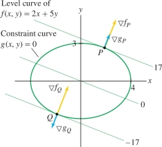
Find the extreme values of \(f(x,y) = 2x+5y\) on the ellipse \[ \left(\frac{x}4\right)^2+\left(\frac{y}3\right)^2= 1 \]

Solution

Step 1. Write out the Lagrange equations.

The constraint curve is \(g(x,y)=0\), where \(g(x,y) =\left({x}/4\right)^2+\left({y}/3\right)^2-1\). We have \[ \nabla f=\left\langle 2, 5\right\rangle,\qquad \nabla g = \left\langle \frac{x}8, \frac{2y}9\right\rangle \]

The Lagrange equations \(\nabla f_P = \lambda \nabla g_P\) are: \begin{equation*} \left\langle 2,5\right\rangle = \lambda \left\langle \frac{x}8, \frac{2y}9\right\rangle\quad\Rightarrow\quad 2 =\frac{\lambda x}8,\qquad 5 = \frac{\lambda (2y)}9\tag{2} \end{equation*}

Step 2. Solve for \(\lambda\) in terms of \(x\) and \(y\).

Eq. (2) gives us two equations for \(\lambda\): \begin{equation*} \lambda = \frac{16}{x},\qquad \lambda = \frac{45}{2 y}\tag{3} \end{equation*}

To justify dividing by \(x\) and \(y\), note that \(x\) and \(y\) must be nonzero, because \(x=0\) or \(y=0\) would violate Eq. (2).

Step 3. Solve for \(x\) and \(y\) using the constraint.

The two expressions for \(\lambda\) must be equal, so we obtain \(\frac{16}{x} = \frac{45}{2 y}\) or \(y = \frac{45}{32}x\). Now substitute this in the constraint equation and solve for \(x\): \[ \begin{array}{rl} \left(\frac{x}4\right)^2+\left(\frac{\frac{45}{32}x}{3}\right)^2 &=1\\ x^2\left(\frac{1}{16}+ \frac{225}{1024}\right)= x^2\left(\frac{289}{1024}\right) &=1 \end{array} \]

Thus \(x=\pm\sqrt{\tfrac{1024}{289}}=\pm \tfrac{32}{17}\), and since \(y = \tfrac{45x}{32}\), the critical points are \(P=\big(\frac{32}{17},\frac{45}{17}\big)\) and \(Q=\big(-\frac{32}{17},-\frac{45}{17}\big)\).

Step 4. Calculate the critical values.

\[ \begin{array}{rl} f(P) &= f\left(\frac{32}{17},\frac{45}{17}\right) = 2\left(\frac{32}{17}\right)+ 5\left(\frac{45}{17}\right) = 17 \end{array} \] and \(f(Q)=-17\). We conclude that the maximum of \(f(x,y)\) on the ellipse is \(17\) and the minimum is \(-17\) (Figure 14.72).

Figure 14.72: The min and max occur where a level curve of \(f\) is tangent to the constraint curve \[ g(x,y)=\left(\frac{x}4\right)^2+\left(\frac{y}3\right)^2-1=0 \]

EXAMPLE 2 Cobb–Douglas Production Function

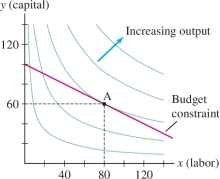
By investing \(x\) units of labor and \(y\) units of capital, a low-end watch manufacturer can produce \(P(x,y) = 50x^{0.4}y^{0.6}\) watches. (See Figure 14.73.) Find the maximum number of watches that can be produced on a budget of $20,000 if labor costs $100 per unit and capital costs $200 per unit.

Figure 14.73: Economist Paul Douglas, working with mathematician Charles Cobb, arrived at the production functions \(P(x,y) = Cx^a y^b\) by fitting data gathered on the relationships between labor, capital, and output in an industrial economy. Douglas was a professor at the University of Chicago and also served as U.S. senator from Illinois from 1949 to 1967.

Solution The total cost of \(x\) units of labor and \(y\) units of capital is \(100x + 200y\). Our task is to maximize the function \(P(x,y) = 50x^{0.4}y^{0.6}\) subject to the following budget constraint (Figure 14.74): \begin{equation*} g(x,y) = 100x+200y-20{,}000=0\tag{4} \end{equation*}

Figure 14.74: Contour plot of the Cobb–Douglas production function \(P(x,y) = 50x^{0.4}y^{0.6}\). The level curves of a production function are called isoquants.

Step 1. Write out the Lagrange equations.

\[ \begin{array}{llll} &P_x(x,y)=\lambda g_x(x,y):&\quad 20x^{-0.6}y^{0.6} &= 100\lambda \\ &P_y(x,y)=\lambda g_y(x,y):&\quad 30x^{0.4}y^{-0.4} &= 200\lambda \end{array} \]

Step 2. Solve for \(\lambda\) in terms of \(x\) and \(y\).

These equations yield two expressions for \(\lambda\) that must be equal: \begin{equation*} \lambda = \frac15\left(\frac{y}x\right)^{0.6} = \frac{3}{20}\left(\frac{y}x\right)^{-0.4}\tag{5} \end{equation*}

Step 3. Solve for \(x\) and \(y\) using the constraint.

Multiply Eq. (5) by \(5(y/x)^{0.4}\) to obtain \(y/x =15/20\), or \(y = \tfrac34 x\). Then substitute in Eq. (4): \[ 100x+200y = 100x+200\left(\frac34 x\right) = 20{,}000\quad\Rightarrow\quad 250x = 20{,}000 \]

We obtain \(x = \tfrac{20{,}000}{250} = 80\) and \(y = \frac34 x = 60\). The critical point is \(A=(80,60)\).

Step 4. Calculate the critical values.

Since \(P(x,y)\) is increasing as a function of \(x\) and \(y\), \(\nabla P\) points to the northeast, and it is clear that \(P(x,y)\) takes on a maximum value at \(A\) (Figure 14.74). The maximum is \(P(80,60)= 50(80)^{0.4}(60)^{0.6} = 3365.87\), or roughly 3365 watches, with a cost per watch of \(\tfrac{20{,}000}{3365}\) or about $5.94.

GRAPHICAL INSIGHT

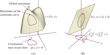
In an ordinary optimization problem without constraint, the global maximum value is the height of the highest point on the surface \(z = f(x,y)\) (point \(Q\) in Figure 14.75). When a constraint is given, we restrict our attention to the curve on the surface lying above the constraint curve \(g(x,y)=0\) . The maximum value subject to the constraint is the height of the highest point on this curve. Figure 14.75 shows the optimization problem solved in Example 1.

EXAMPLE 3 Lagrange Multipliers in Three Variables

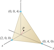
Find the point on the plane \(\frac{x}2+\frac{y}4+\frac{z}4=1\) closest to the origin in \({\bf{R}}^3\).

Solution Our task is to minimize the distance \(d=\sqrt{x^2+y^2+z^2}\) subject to the constraint \(\dfrac{x}2+\dfrac{y}4+\dfrac{z}4=1\). But finding the minimum distance \(d\) is the same as finding the minimum square of the distance \(d^2\), so our problem can be stated: \[ \textrm{Minimize } f(x,y,z)=x^2+y^2+z^2\quad\textrm{subject to }\quad g(x,y,z)=\dfrac{x}2+\dfrac{y}4+\dfrac{z}4-1=0 \]

The Lagrange condition is \[ \underbrace{\left\langle 2x, 2y, 2z\right\rangle}_{\nabla f} = \lambda \underbrace{\left\langle \frac12, \frac14, \frac14 \right\rangle}_{\nabla g} \]

This yields \[ \lambda = 4x=8y=8z\quad\Rightarrow\quad z=y=\frac x2 \]

Substituting in the constraint equation, we obtain \[ \frac{x}2+\frac{y}4+\frac{z}4= \frac{2z}2+\frac{z}4+\frac{z}4= \frac{3z}2= 1\quad \Rightarrow\quad z=\frac23 \]

Thus, \(x = 2z=\tfrac{4}{3}\) and \(y =z=\tfrac23\). This critical point must correspond to the minimum of \(f\) (because \(f\) has no maximum on the constraint plane). Hence, the point on the plane closest to the origin is \(P=\big(\frac43,\frac23,\frac23\big)\) (Figure 14.76).

Figure 14.76: Point \(P\) closest to the origin on the plane.

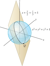
The intersection of a sphere with a plane through its center is called a great circle.

EXAMPLE 4 Lagrange Multipliers with Multiple Constraints

The intersection of the plane \(x+\tfrac12y+\tfrac13z=0\) with the unit sphere \(x^2+y^2+z^2=1\) is a great circle (Figure 14.77). Find the point on this great circle with the largest \(x\) coordinate.

Solution Our task is to maximize the function \(f(x,y,z)=x\) subject to the two constraint equations \[ g(x,y,z) = x+\frac12y+\frac13z = 0,\qquad h(x,y,z) = x^2+y^2+z^2-1 = 0 \]

Figure 14.77: The plane intersects the sphere in a great circle. \(Q\) is the point on this great circle with the largest \(x\)-coordinate.

The Lagrange condition is \[ \begin{array}{rl} \nabla f &= \lambda\nabla g + \mu\nabla h\\ \left\langle 1,0,0\right\rangle &= \lambda\left\langle 1,\frac12, \frac13 \right\rangle +\mu \left\langle 2x, 2y, 2z\right\rangle \end{array} \]

Note that \(\mu\) cannot be zero. The Lagrange condition would become \(\left\langle 1,0,0\right\rangle = \lambda \big\langle 1, \frac12, \frac13\big\rangle\), and this equation is not satisfed for any value of \(\lambda\). Now, the Lagrange condition gives us three equations: \[ \lambda+2\mu x = 1,\qquad \frac12\lambda+2\mu y=0,\qquad \frac13\lambda +2\mu z = 0 \]

The last two equations yield \(\lambda = -4\mu y\) and \(\lambda = -6\mu z\). Because \(\mu \neq 0\), \[ -4\mu y = -6\mu z\quad\Rightarrow\quad \boxed{y = \frac32 z} \]

Now use this relation in the first constraint equation: \[ x+\frac12y+\frac13z = x + \frac12\left(\frac32 z\right) + \frac13z = 0\quad\Rightarrow\quad \boxed{ x = -\frac{13}{12}z} \]

Finally, we can substitute in the second constraint equation: \[ x^2+y^2+z^2-1 = \left(-\frac{13}{12}z\right)^2 + \left(\frac32 z\right)^2 +z^2 - 1= 0 \] to obtain \(\tfrac{637}{144}z^2=1\) or \(z=\pm \tfrac{12}{7\sqrt{13}}\). Since \(x = -\frac{13}{12}z\) and \(y = \frac32 z\), the critical points are \[ P= \left(-\frac{\sqrt{13}}{7}, \frac{18}{7\sqrt{13}}, \frac{12}{7\sqrt{13}}\right),\qquad Q= \left(\frac{\sqrt{13}}{7}, -\frac{18}{7\sqrt{13}}, -\frac{12}{7\sqrt{13}}\right) \]

The critical point with the largest \(x\)-coordinate (the maximum value of \(f(x,y,z)\)) is \(Q\) with \(x\)-coordinate \(\tfrac{\sqrt{13}}{7}\approx 0.515\).