15.3 Triple Integrals
Triple integrals of functions \(f(x,y,z)\) of three variables are a fairly straightforward generalization of double integrals. Instead of a rectangle in the plane, our domain is a box Figure 15.32 \[ {\mathcal{B}} = [a,b]\times[c,d]\times [p,q] \] consisting of all points \((x,y,z)\) in \({\bf{R}}^3\) such that \[ a\le x \le b,\qquad c\le y \le d,\qquad p\le z\le q \]
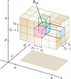
To integrate over this box, we subdivide the box (as usual) into “sub”-boxes \[ {\mathcal{B}}_{ijk} = [x_{i-1}, x_i] \times [y_{j-1}, y_j] \times [z_{k-1}, z_k] \] by choosing partitions of the three intervals \[ \begin{array}{rcl} a &=& x_0 < x_1 < \cdots < x_N = b\\ c &=& y_0 < y_1 < \cdots < y_M = d\\ p &=& z_0 < z_1 < \cdots < z_L = q \end{array} \]
Here \(N, M,\) and \(L\) are positive integers. The volume of \({\mathcal{B}}_{ijk}\) is \(\Delta V_{ijk} = \Delta x_i\, \Delta y_j\, \Delta z_k\) where \[ \Delta x_i = x_i - x_{i - 1},\qquad \Delta y_j = y_j - y_{j - 1},\qquad \Delta z_k = z_k - z_{k - 1} \]
886
Then, we choose a sample point \(P_{ijk}\) in each box \({\mathcal{B}}_{ijk}\) and form the Riemann sum \[ S_{N,M,L} = \sum_{i=1}^N \sum_{j=1}^M\sum_{k=1}^L f(P_{ijk})\,\Delta V_{ijk} \]
As in the previous section, we write \({\mathcal{P}}=\{\{x_i\},\{y_j\},\{z_k\}\}\) for the partition and let \(\left \| {{\mathcal{P}}} \right \|\) be the maximum of the widths \(\Delta x_i, \Delta y_j, \Delta z_k\). If the sums \(S_{N,M,L}\) approach a limit as \(\left \| {{\mathcal{P}}} \right \| \to 0\) for arbitrary choices of sample points, we say that \(f\) is integrable over \({\mathcal{B}}\). The limit value is denoted \[ \iiint_{{\mathcal{B}}\,} f(x,y,z)\,dV = \lim_{\left \| {{\mathcal{P}}} \right \| \to 0} S_{N,M,L} \]
Triple integrals have many of the same properties as double and single integrals. The linear properties are satisfied, and continuous functions are integrable over a box \({\mathcal{B}}\). Furthermore, triple integrals can be evaluated as iterated integrals.
The notation \(d\!A\), used in the previous section, suggests area and occurs in double integrals over domains in the plane. Similarly, \(dV\) suggests volume and is used in the notation for triple integrals.
THEOREM 1 Fubini’s Theorem for Triple Integrals
The triple integral of a continuous function \(f(x,y,z)\) over a box \({\mathcal{B}} = [a,b]\times[c,d]\times [p,q]\) is equal to the iterated integral: \[ \boxed{\iiint_{{\mathcal{B}}\,} f(x,y,z)\,dV = \int_{x=a}^b\int_{y=c}^d \int_{z=p}^q f(x,y,z)\,dz\,dy\,dx} \]
Furthermore, the iterated integral may be evaluated in any order.
As noted in the theorem, we are free to evaluate the iterated integral in any order (there are six different orders). For instance, \[ \int_{x=a}^b\int_{y=c}^d \int_{z=p}^q f(x,y,z)\,dz\,dy\,dx = \int_{z=p}^q\int_{y=c}^d \int_{x=a}^b f(x,y,z)\,dx\,dy\,dz \]
EXAMPLE 1 Integration over a Box
Calculate the integral \(\iiint_{{\mathcal{B}}\,} x^2e^{y+3z} \,dV\), where \({\mathcal{B}} = [1,4]\times[0,3]\times [2,6]\).
Solution We write this triple integral as an iterated integral: \[ \iiint_{{\mathcal{B}}\,} x^2e^{y+3z} \,dV = \int_1^4\int_0^3\int_2^6 x^2e^{y+3z} \,dz\,dy\,dx \]
Step 1. Evaluate the inner integral with respect to \(z\), holding \(x\) and \(y\) constant.
\[ \int_{z=2}^6 x^2e^{y+3z} \,dz = \frac13 x^2e^{y+3z}\bigg|_2^6 = \frac13 x^2e^{y+18}-\frac13 x^2e^{y+6} = \frac13(e^{18}-e^6)x^2e^y \]
Step 2. Evaluate the middle integral with respect to \(y\), holding \(x\) constant.
\[ \int_{y=0}^3 \frac13(e^{18}-e^6)x^2e^y\,dy = \frac13 (e^{18}-e^6)x^2\int_{y=0}^3e^y\,dy = \frac13 (e^{18}-e^6)(e^3-1)x^2 \]
Step 3. Evaluate the outer integral with respect to \(x\).
\[ \iiint_{{\mathcal{B}}\,} (x^2e^{y+3z})\,dV = \frac13(e^{18}-e^6)(e^3-1) \int_{x=1}^4 x^2\,dx = 7(e^{18}-e^6)(e^3-1) \]
887
Note that in the previous example, the integrand factors as a product of three functions \(f(x,y,z) = g(x)h(y)k(z)\)—namely, \[ f(x,y,z) = x^2 e^{y+3z} = x^2 e^y e^{3z} \]
Because of this, the triple integral can be evaluated simply as the product of three single integrals: \[ \begin{array}{rl} \iiint_{{\mathcal{B}}\,} x^2 e^y e^{3z}\,dV &= \left(\int_1^4 x^2\,dx\right) \left(\int_0^3 e^y\,dy\right) \left(\int_2^6 e^{3z}\,dz\right)\\ &= (21)(e^3 - 1)\left(\frac{e^{18} - e^6}{3}\right) = 7(e^{18}-e^6)(e^3-1) \end{array} \]
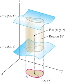
Next, instead of a box, we integrate over a solid region \({\mathcal{W}}\) that is simple as in Figure 15.33. In other words, \({\mathcal{W}}\) is the region between two surfaces \(z = z_1(x,y)\) and \(z = z_2(x,y)\) over a domain \({\mathcal{D}}\) in the \(xy\)-plane. In this case, \begin{equation*} {\mathcal{W}} = \{(x,y,z): (x,y)\in {\mathcal{D}}\quad \textrm{and}\quad z_1(x,y)\le z \le z_2 (x,y)\}\tag{1} \end{equation*}
The domain \({\mathcal{D}}\) is the projection of \({\mathcal{W}}\) onto the \(xy\)-plane.
As a formal matter, as in the case of double integrals, we define the triple integral of \(f(x,y,z)\) over \({\mathcal{W}}\) by \[ \iiint_{{\mathcal{W}}\,} f(x,y,z)\,dV = \iiint_{{\mathcal{B}}\,} \tilde{f}(x,y,z)\,dV \] where \({\mathcal{B}}\) is a box containing \({\mathcal{W}}\), and \(\tilde{f}\) is the function that is equal to \(f\) on \({\mathcal{W}}\) and equal to zero outside of \({\mathcal{W}}\). The triple integral exists, assuming that \(z_1(x,y)\), \(z_2(x,y)\), and the integrand \(f\) are continuous. In practice, however, we evaluate triple integrals as iterated integrals. This is justified by the following theorem, whose proof is similar to that of Theorem 2 in Section 15.2.
THEOREM 2
The triple integral of a continuous function \(f\) over the region \[ {\mathcal{W}}: (x,y)\in {\mathcal{D}},\quad z_1(x,y)\le z \le z_2(x,y) \] is equal to the iterated integral \[ \boxed{\iiint_{{\mathcal{W}}\,} f(x,y,z) \,dV = \iint_{{\mathcal{D}}\,}\left( \int_{z= z_1(x,y)}^{z_2(x,y)} f(x,y,z)\,dz\right)dA } \]
More generally, integrals of functions of \(n\) variables (for any \(n\)) arise naturally in many different contexts. For example, the average distance between two points in a ball is expressed as a six-fold integral because we integrate over all possible coordinates of the two points. Each point has three coordinates for a total of six variables.
One thing missing from our discussion so far is a geometric interpretation of triple integrals. A double integral represents the signed volume of the three-dimensional region between a graph \(z = f(x,y)\) and the \(xy\)-plane. The graph of a function \(f(x,y,z)\) of three variables lives in four-dimensional space, and thus a triple integral represents a four-dimensional volume. This volume is hard or impossible to visualize. On the other hand, triple integrals represent many other types of quantities. Some examples are total mass, average value, probabilities, and centers of mass (see Section 15.5).
Furthermore, the volume \(V\) of a region \({\mathcal{W}}\) is defined as the triple integral of the constant function \(f(x,y,z)=1\): \[ \boxed{V = \iiint_{\mathcal{W}}\, 1\,dV} \]
888
In particular, if \({\mathcal{W}}\) is a simple region between \(z=z_1(x,y)\) and \(z=z_2(x,y)\), then \[ \iiint_{{\mathcal{W}}\,} 1\,dV = \iint_{{\mathcal{D}}\,}\left( \int_{z=z_1(x,y)}^{z_2(x,y)} 1\,dz\right)dA = \iint_{{\mathcal{D}}\,}\left(z_2(x,y) - z_1(x,y) \right)dA \]
Thus, the triple integral is equal to the double integral defining the volume of the region between the two surfaces.
EXAMPLE 2 Solid Region with a Rectangular Base
Evaluate \(\iiint_{{\mathcal{W}}\,} z\,dV\), where \({\mathcal{W}}\) is the region between the planes \(z=x+y\) and \(z=3x+5y\) lying over the rectangle \({\mathcal{D}}=[0,3]\times[0,2]\) Figure 15.34.
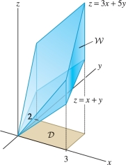
Solution Apply Theorem 2 with \(z_1(x,y)=x+y\) and \(z_2(x,y)=3x+5y\): \[ \iiint_{{\mathcal{W}}\,} z \,dV = \iint_{{\mathcal{D}}\,}\left(\int_{z=x+y}^{3x+5y} z \,dz\right)dA= \int_{x=0}^3\int_{y=0}^2 \int_{z=x+y}^{3x+5y} z \,dz\,dy\,dx \]
Step 1. Evaluate the inner integral with respect to \(z\).
\begin{equation*} \int_{z=x+y}^{3x+5y} z \,dz = \frac12z^2\bigg|_{z=x+y}^{3x+5y} = \frac12(3x+5y)^2-\frac12(x+y)^2 = 4x^2+14xy+12y^2\tag{2} \end{equation*}
Step 2. Evaluate the result with respect to \(y\).
\[ \int_{y=0}^2 (4x^2+14xy+12y^2) \,dy =(4x^2y+7xy^2+4y^3)\bigg|_{y=0}^2 = 8x^2+28x+32 \]
Step 3. Evaluate the result with respect to \(x\).
\[ \begin{array}{rl} \iiint_{{\mathcal{W}}\,} z \,dV &= \int_{x=0}^3( 8x^2+28x+32)\,dx = \left(\frac{8}3x^3 +14x^2+32x\right)\bigg|_0^3 \\ &= 72 + 126+ 96 = 294 \end{array} \]
EXAMPLE 3 Solid Region with a Triangular Base
Evaluate \(\iiint_{{\mathcal{W}}\,} z\,dV\), where \({\mathcal{W}}\) is the region in Figure 15.35.
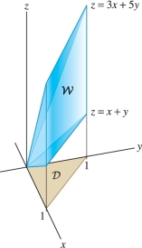
Solution This is similar to the previous example, but now \({\mathcal{W}}\) lies over the triangle \({\mathcal{D}}\) in the \(xy\)-plane defined by \[ 0\le x \le 1,\qquad 0 \le y \le 1-x \]
Thus, the triple integral is equal to the iterated integral: \[ \begin{array}{rl} \iiint_{{\mathcal{W}}\,} z \,dV &= \iint_{{\mathcal{D}}\,}\left( \int_{z=x+y}^{3x+5y} z \,dz\right)dA= \underbrace{\int_{x=0}^1\int_{y=0}^{1-x}}_{ \mbox{Integral} \atop \mbox{over triangle}} \int_{z=x+y}^{3x+5y} z \,dz\, dy\,dx \end{array} \]
We computed the inner integral in the previous example [see Eq. (2)]: \[ \int_{z=x+y}^{3x+5y} z \,dz = \frac12z^2\bigg|_{x+y}^{3x+5y} =4x^2+14xy+12y^2 \]
889
Next, we integrate with respect to \(y\): \[ \begin{array}{rl} \int_{y=0}^{1-x} (4x^2+14xy+12y^2) \,dy &= ( 4x^2y+7xy^2+4y^3)\bigg|_{y=0}^{1-x} \\ & = 4x^2(1-x)+7x(1-x)^2+4(1-x)^3 \\ &= 4-5x+2x^2-x^3 \end{array} \]
And finally, \[ \begin{array}{rl} \iiint_{{\mathcal{W}}\,} z \,dV &= \int_{x=0}^1(4-5x+2x^2-x^3)\,dx\\ & = 4-\frac52+\frac23-\frac14 = \frac{23}{12} \end{array} \]
EXAMPLE 4 Region between Intersecting Surfaces
Integrate \(f(x,y,z)=x\) over the region \({\mathcal{W}}\) bounded above by \(z=4- x^2-y^2\) and below by \(z= x^2+3y^2\) in the octant \(x \ge 0, y\ge0, z\ge 0\).
Solution The region \({\mathcal{W}}\) is simple, so \[ \iiint_{{\mathcal{W}}\,} x \,dV = \iint_{{\mathcal{D}}\,} \int_{z=x^2+3y^2}^{4-x^2-y^2} x\,dz\,dA \] where \({\mathcal{D}}\) is the projection of \({\mathcal{W}}\) onto the \(xy\)-plane. To evaluate the integral over \({\mathcal{D}}\), we must find the equation of the curved part of the boundary of \({\mathcal{D}}\).
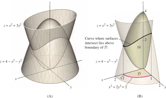
Step 1. Find the boundary of \({\mathcal{D}}\).
The upper and lower surfaces intersect where they have the same height: \[ z= x^2+3y^2 = 4- x^2-y^2\qquad \textrm{or}\qquad x^2+2y^2=2 \]
Therefore, as we see in Figure 15.36, \({\mathcal{W}}\) projects onto the domain \({\mathcal{D}}\) consisting of the quarter of the ellipse \(x^2+2y^2 = 2\) in the first quadrant. This ellipse hits the axes at \((\sqrt{2},0)\) and \((0,1)\).
890
Step 2. Express \({\mathcal{D}}\) as a simple domain.
We can integrate in either the order \(dy\,dx\) or \(dx\,dy\). If we choose \(dx\,dy\), then \(y\) varies from \(0\) to \(1\) and the domain is described by \[ {\mathcal{D}}: 0\le y \le 1,\quad 0 \le x\le \sqrt{2-2y^2} \]
Step 3. Write the triple integral as an iterated integral.
\[ \iiint_{{\mathcal{W}}\,} x \,dV = \int_{y=0}^1\int_{x=0}^{\sqrt{2-2y^2}}\int_{z= x^2+3y^2}^{4-x^2-y^2} x\,dz\,dx\,dy \]
Step 4. Evaluate.
Here are the results of evaluating the integrals in order:
- Inner integral: \(\int_{z= x^2 + y^2}^{4-x^2-y^2} x \,dz = xz\bigg|_{z= x^2+3y^2}^{4-x^2-y^2} = 4x-2x^3-4y^2x\)
- Middle integral: \[ \begin{array}{rcl} \int_{x=0}^{\sqrt{2-2y^2}} (4x-2x^3-4y^2x)\,dx &=& \left( 2x^2-\frac12x^4-2x^2y^2 \right)\bigg|_{x=0}^{\sqrt{2-2y^2}}\\ &=& 2 - 4 y^2 + 2y^4 \end{array} \]
- Triple integral: \(\iiint_{{\mathcal{W}}\,} x \,dV = \int_0^1(2 - 4 y^2 + 2y^4)\,dy = 2-\frac43+\frac25 =\frac{16}{15}\)
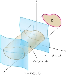
So far, we have evaluated triple integrals by projecting the region \({\mathcal{W}}\) onto a domain \({\mathcal{D}}\) in the \(xy\)-plane. We can integrate equally well by projecting onto domains in the \(xz\)- or \(yz\)-plane. For example, if \({\mathcal{W}}\) is the simple region between the graphs of \(x=x_1(y,z)\) and \(x=x_2(y,z)\) lying over a domain \({\mathcal{D}}\) in the \(yz\)-plane Figure 15.37, then \[ \iiint_{{\mathcal{W}}\,} f(x,y,z)\,dV = \iint_{{\mathcal{D}}\,}\left(\int_{x=x_1(y,z)}^{x_2(y,z)}f(x,y,z)\,dx\right) dA \]
EXAMPLE 5 Writing a Triple Integral in Three Ways
The region \({\mathcal{W}}\) in Figure 15.38 is bounded by \[ z=4-y^2,\qquad y=2x,\qquad z=0,\qquad x=0 \]
Express \(\iiint_{{\mathcal{W}}\,} xyz\,dV\) as an iterated integral in three ways, by projecting onto each of the three coordinate planes (but do not evaluate).
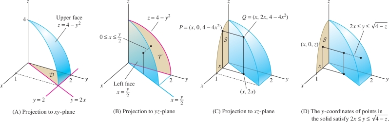
Solution We consider each coordinate plane separately.
You can check that all three ways of writing the triple integral in Example 5 yield the same answer: \[ \iiint_{{\mathcal{W}}} xyz\,dV = \frac23 \]
Step 1. The \(xy\)-plane.
The upper face \(z=4-y^2\) intersects the first quadrant of the \(xy\)-plane (\(z=0\)) in the line \(y=2\) [Figure 15.38]. Therefore, the projection of \({\mathcal{W}}\) onto the \(xy\)-plane is a triangle \({\mathcal{D}}\) defined by \(0\le x \le 1\), \(2x\le y \le 2\), and \[ \displaystyle{\mathcal{W}}:0\le x \le 1,\quad 2x\le y \le 2,\quad 0\le z \le 4-y^2 \] \begin{equation*} \displaystyle\iiint_{{\mathcal{W}}\,} xyz\,dV = \int_{x=0}^1\int_{y=2x}^{2}\int_{z=0}^{4-y^2} xyz\,dz\,dy\,dx\tag{3} \end{equation*}
891
Step 2. The \(yz\)-plane.
The projection of \({\mathcal{W}}\) onto the \(yz\)-plane is the domain \(\mathcal T\) [Figure 15.38]: \[ {\mathcal T}: 0\le y \le 2,\quad 0 \le z \le 4-y^2 \]
The region \({\mathcal{W}}\) consists of all points lying between \(\mathcal T\) and the “left face” \(x=\frac12y\). In other words, the \(x\)-coordinate must satisfy \(0 \le x \le \tfrac12y\). Thus, \[ \begin{array}{c} \displaystyle {\mathcal{W}}: 0\le y \le 2,\quad 0\le z \le 4-y^2,\qquad 0\le x \le \frac12y\\ \displaystyle \iiint_{{\mathcal{W}}\,} xyz\,dV=\int_{y=0}^2\int_{z=0}^{4-y^2}\int_{x=0}^{y/2} xyz\,dx\,dz\,dy \end{array} \]
Step 3. The \(xz\)-plane.
The challenge in this case is to determine the projection of \({\mathcal{W}}\) onto the \(xz\)-plane, that is, the region \(S\) in Figure 15.38. We need to find the equation of the boundary curve of \(S\). A point \(P\) on this curve is the projection of a point \(Q = (x,y,z)\) on the boundary of the left face. Since \(Q\) lies on both the plane \(y=2x\) and the surface \(z=4-y^2\), \(Q=(x,2x,4-4x^2)\). The projection of \(Q\) is \(P=(x,0,4-4x^2)\). We see that the projection of \({\mathcal{W}}\) onto the \(xz\)-plane is the domain \[ S: 0\le x \le 1,\quad 0\le z \le 4-4x^2 \]
This gives us limits for \(x\) and \(z\) variables, so the triple integral can be written \[ \iiint_{{\mathcal{W}}\,} xyz\,dV=\int_{x=0}^1\int_{z=0}^{4-4x^2}\int_{y=??}^{??} xyz\,dy\,dz\,dx \]
What are the limits for \(y\)? The equation of the upper face \(z=4-y^2\) can be written \(y=\sqrt{4-z}\). Referring to Figure 15.38, we see that \({\mathcal{W}}\) is bounded by the left face \(y=2x\) and the upper face \(y=\sqrt{4-z}\). In other words, the \(y\)-coordinate of a point in \({\mathcal{W}}\) satisfies \[ 2x\le y \le \sqrt{4-z} \]
Now we can write the triple integral as the following iterated integral: \[ \iiint_{{\mathcal{W}}\,} xyz\,dV=\int_{x=0}^1\int_{z=0}^{4-4x^2}\int_{y=2x}^{\sqrt{4-z}} xyz\,dy\,dz\,dx \]
892
The average value of a function of three variables is defined as in the case of two variables: \begin{equation*} \overline{f} = \frac1{\textrm{Volume}({\mathcal{W}})} \iiint_{{\mathcal{W}}\,} f(x,y,z)\,dV\tag{4} \end{equation*} where \(\text{Volume}({\mathcal{W}}) = \iiint_{{\mathcal{W}}\,} 1\,dV\). And, as in the case of two variables, \(\overline{f}\) lies between the minimum and maximum values of \(f\) on \({\mathcal{D}}\), and the Mean Value Theorem holds: If \({\mathcal{W}}\) is connected and \(f\) is continuous on \({\mathcal{W}}\), then there exists a point \(P\in{\mathcal{W}}\) such that \(f(P)=\overline{f}\).
Excursion: Volume of the Sphere in Higher Dimensions
Archimedes (287–212 BCE) proved the beautiful formula \(V=\frac43\pi r^3\) for the volume of a sphere nearly 2000 years before calculus was invented, by means of a brilliant geometric argument showing that the volume of a sphere is equal to two-thirds the volume of the circumscribed cylinder. According to Plutarch (ca. 45–120 CE), Archimedes valued this achievement so highly that he requested that a sphere with circumscribed cylinder be engraved on his tomb.
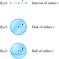
We can use integration to generalize Archimedes' formula to \(n\) dimensions. The ball of radius \(r\) in \({\bf{R}}^n\), denoted \(B_n(r)\), is the set of points \((x_1, \ldots , x_n)\) in \({\bf{R}}^n\) such that \[ x_1^2+x_2^2+\cdots + x_n^2 \le r^2 \]
The balls \(B_n(r)\) in dimensions 1, 2, and 3 are the interval, disk, and ball shown in Figure 15.39. In dimensions \(n \ge 4\), the ball \(B_n(r)\) is difficult, if not impossible, to visualize, but we can compute its volume. Denote this volume by \(V_n(r)\). For \(n=1\), the “volume” \(V_1(r)\) is the length of the interval \(B_1(r)\), and for \(n=2\), \(V_2(r)\) is the area of the disk \(B_2(r)\). We know that \[ V_1(r)=2r,\qquad V_2(r)=\pi r^2,\qquad V_3(r) = \frac43\pi r^3 \]
For \(n\ge 4\), \(V_n(r)\) is sometimes called the hypervolume.
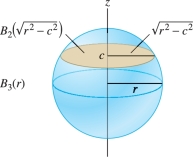
The key idea is to determine \(V_n(r)\) from the formula for \(V_{n-1}(r)\) by integrating cross-sectional volume. Consider the case \(n=3\), where the horizontal slice at height \(z=c\) is a two-dimensional ball (a disk) of radius \(\sqrt{r^2-c^2}\) Figure 15.40. The volume \(V_3(r)\) is equal to the integral of these horizontal slices: \[ V_3(r) = \int_{z =-r}^r V_2 \left(\sqrt{r^2-z^2}\right)\,dz = \int_{z =-r}^r \pi(r^2-z^2)\,dz = \frac43\,\pi r^3 \]
By induction, we can show that for all \(n \ge 1\), there is a constant \(A_n\) (equal to the volume of the \(n\)-dimensional unit ball) such that \begin{equation*} \boxed{V_n(r) = A_n r^n}\tag{5} \end{equation*}
The slice of \(B_n(r)\) at height \(x_n = c\) has equation \[ x_1^2+x_2^2+\cdots + x_{n-1}^2+c^2=r^2 \]
This slice is the ball \(B_{n-1}\bigl(\sqrt{r^2-c^2}\bigr)\) of radius \(\sqrt{r^2 - c^2}\), and \(V_n(r)\) is obtained by integrating the volume of these slices: \[ V_n(r) = \int_{x_n =-r}^r V_{n-1}\left(\sqrt{r^2-x_n^2}\right)\,dx_n = A_{n-1} \int_{x_n =-r}^r \left(\sqrt{r^2-x_n^2}\right)^{n-1}\,dx_n \]
893
Using the substitution \(x_n = r\sin\theta\) and \(dx_n=r\cos\theta\,d\theta\), we have \[ V_n(r) = A_{n-1}r^n\int_{-\pi/2}^{\pi/2} \cos^n\theta\,d\theta = A_{n-1}C_nr^n \] where \(C_n = \displaystyle \int_{\theta = -\pi/2}^{\pi/2} \cos^n\theta\,d\theta\). This proves Eq. (5) with \begin{equation*} \boxed{A_n = A_{n-1}C_n}\tag{6} \end{equation*}
In Exercise 39, you are asked to use Integration by Parts to verify the relation \begin{equation*} C_n = \left(\frac{n-1}n\right) C_{n-2}\tag{7} \end{equation*}
It is easy to check directly that \(C_0=\pi\) and \(C_1=2\). By Eq.(7), \(C_2=\frac12 C_0=\frac{\pi}{2}\), \(C_3=\frac23(2)=\frac43\), and so on. Here are the first few values of \(C_n\):
| \(n\) | 0 | 1 | 2 | 3 | 4 | 5 | 6 | 7 |
| \(C_n\) | \(\pi\) | 2 | \(\tfrac{\pi}2\) | \(\tfrac43\) | \(\frac{3\pi}8\) | \(\tfrac{16}{15}\) | \(\frac{5\pi}{16}\) | \(\tfrac{32}{35}\) |
We also have \(A_1=2\) and \(A_2=\pi\), so we can use the values of \(C_n\) together with Eq. (6 ) to obtain the values of \(A_n\) in Table 15.1. We see, for example, that the ball of radius \(r\) in four dimensions has volume \(V_4(r)=\frac12\pi^2r^4\). The general formula depends on whether \(n\) is even or odd. Using induction and formulas (6) and (7), we can prove that \[ \boxed{ A_{2m} = \frac{\pi^m}{m!},\qquad A_{2m+1} = \frac{2^{m+1}\pi^m}{1\cdot 3\cdot 5 \cdot\cdots\cdot (2m+1)}} \]
| \(n\) | \(A_n\) |
|---|---|
| 1 | 2 |
| 2 | \(\pi\approx 3.14\) |
| 3 | \(\tfrac43 \pi\approx 4.19\) |
| 4 | \(\tfrac{\pi^2}2\approx 4.93\) |
| 5 | \(\mathbf{\tfrac{8\pi^2}{15}\approx 5.26}\) |
| 6 | \(\tfrac{\pi^3}{6}\approx 5.17\) |
| 7 | \(\tfrac{16\pi^3}{105}\approx 4.72\) |
This sequence of numbers \(A_n\) has a curious property. Setting \(r=1\) in Eq. (5), we see that \(A_n\) is the volume of the unit ball in \(n\) dimensions. From Table 15.1, it appears that the volumes increase up to dimension \(5\) and then begin to decrease. In Exercise 40, you are asked to verify that the five-dimensional unit ball has the largest volume. Furthermore, the volumes \(A_n\) tend to 0 as \(n\to\infty\).
15.3.1 Summary
- The triple integral over a box \({\mathcal{B}} = [a,b]\times[c,d]\times [p,q]\) is equal to the iterated integral \[ \iiint_{{\mathcal{B}}\,} f(x,y,z)\,dV = \int_{x=a}^b\int_{y=c}^d \int_{z=p}^q f(x,y,z)\,dz\,dy\,dx \] The iterated integral may be written in any one of six possible orders—for example, \[ \int_{z=p}^q\int_{y=c}^d \int_{x=a}^b f(x,y,z)\,dx\,dy\,dz \]
- A simple region \({\mathcal{W}}\) in \({\bf{R}}^3\) is a region consisting of the points \((x,y,z)\) between two surfaces \(z=z_1(x,y)\) and \(z=z_2(x,y)\), where \(z_1(x,y) \leq z_2(x,y)\), lying over a domain \({\mathcal{D}}\) in the \(xy\)-plane. In other words, \({\mathcal{W}}\) is defined by \[ (x,y)\in {\mathcal{D}},\qquad z_1(x,y)\le z \le z_2(x,y) \] The triple integral over \({\mathcal{W}}\) is equal to an iterated integral: \[ \iiint_{{\mathcal{W}}\,} f(x,y,z) \,dV = \iint_{{\mathcal{D}}\,}\left(\int_{z=z_1(x,y)}^{z_2(x,y)} f(x,y,z)\,dz\right)dA \]
- The average value of \(f(x,y,z)\) on a region \({\mathcal{W}}\) of volume \(V\) is the quantity \[ \overline{f}=\frac1V \iiint_{{\mathcal{W}}\,} f(x,y,z)\,dV,\qquad V=\iiint_{{\mathcal{W}}\,}1\,dV \]
894