15.6 Change of Variables
The formulas for integration in polar, cylindrical, and spherical coordinates are important special cases of the general Change of Variables Formula for multiple integrals. In this section we discuss the general formula.
Maps from \({\bf{R}}^2\) to \({\bf{R}}^2\)
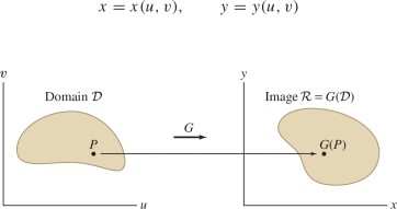
A function \({G}: X\to Y\) from a set \(X\) (the domain) to another set \(Y\) is often called a map or a mapping. For \(x\in X\), the element \({G}(x)\) belongs to \(Y\) and is called the image of \(x\). The set of all images \({G}(x)\) is called the image or range of \({G}\). We denote the image by \({G}(X)\).
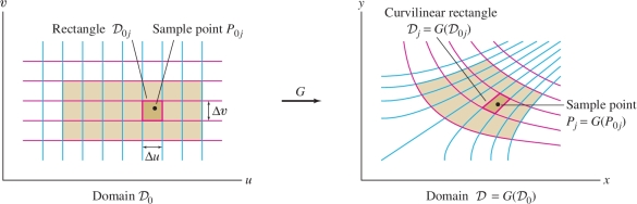
In this section, we consider maps \({G}:{\mathcal{D}} \to{\bf{R}}^2\) defined on a domain \({\mathcal{D}}\) in \({\bf{R}}^2\) Figure 15.66. To prevent confusion, we'll often use \(u\), \(v\) as our domain variables and \(x\), \(y\) for the range. Thus, we will write \({G}(u,v) = ({x}(u,v),{y}(u,v))\), where the components \({x}\) and \({y}\) are functions of \(u\) and \(v\): \[ x = {x}(u,v),\qquad y = {y}(u,v) \]
One map we are familiar with is the map defining polar coordinates. For this map, we use variables \(r, \theta\) instead of \(u, v\). The polar coordinates map \({G}: {\bf{R}}^2\to{\bf{R}}^2\) is defined by \[ {G}(r,\theta) = (r\cos\theta,r\sin\theta) \]
EXAMPLE 1 Polar Coordinates Map
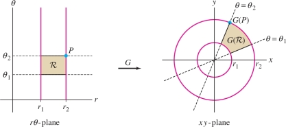
Describe the image of a polar rectangle \({\mathcal{R}} = [r_1,r_2]\times [\theta_1,\theta_2]\) under the polar coordinates map.
Solution Referring to Figure 15.67, we see that:
- A vertical line \(r=r_1\) (shown in red) is mapped to the set of points with radial coordinate \(r_1\) and arbitrary angle. This is the circle of radius \(r_1\).
- A horizontal line \(\theta=\theta_1\) (dashed line in the figure) is mapped to the set of points with polar angle \(\theta\) and arbitrary \(r\)-coordinate. This is the line through the origin of angle \(\theta_1\).
The image of \({\mathcal{R}} = [r_1,r_2]\times [\theta_1,\theta_2]\) under the polar coordinates map \(G(r,\theta) = (r\cos\theta, r\sin\theta)\) is the polar rectangle in the \(xy\)-plane defined by \(r_1\le r \le r_2\), \(\theta_1\le \theta \le \theta_2\).
921
General mappings can be quite complicated, so it is useful to study the simplest case—linear maps—in detail. A map \({G}(u,v)\) is linear if it has the form \[ {G}(u,v) = ( Au+Cv, Bu+Dv)\quad (A, B, C, D~\textrm{constants}) \]
We can get a clear picture of this linear map by thinking of \(G\) as a map from vectors in the \(uv\)-plane to vectors in the \(xy\)-plane. Then \({G}\) has the following linearity properties (see Exercise 46): \begin{equation*} {G}(u_1+u_2,v_1+v_2)={G}(u_1,v_1)+{G}(u_2,v_2)\tag{1} \end{equation*} \begin{equation*} {G}(cu,cv)=c{G}(u,v)\quad (c\hbox{ any constant)}\tag{2} \end{equation*}
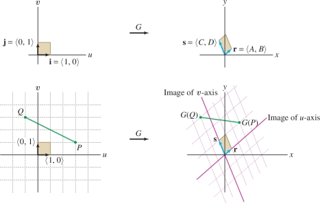
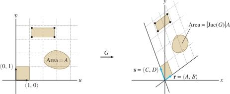
A consequence of these properties is that \({G}\) maps the parallelogram spanned by any two vectors \({\bf{a}}\) and \({\bf{b}}\) in the \(uv\)-plane to the parallelogram spanned by the images \({G}({\bf{a}})\) and \({G}({\bf{b}})\), as shown in Figure 15.68.
More generally, \({G}\) maps the segment joining any two points \(P\) and \(Q\) to the segment joining \({G}(P)\) and \({G}(Q)\) (see Exercise 47). The grid generated by basis vectors \({\bf{i}}=\left\langle 1,0\right\rangle\) and \({\bf{j}}=\left\langle 0,1\right\rangle\) is mapped to the grid generated by the image vectors Figure 15.68 \[ \begin{array}{rl} {\bf{r}} &= {G}( 1,0 )=\left\langle A,B \right\rangle\\ {\bf{s}} &= {G}( 0,1 )=\left\langle C,D \right\rangle \end{array} \]
922
EXAMPLE 2 Image of a Triangle
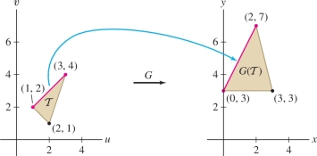
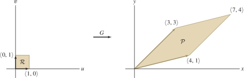
Find the image of the triangle \(\mathcal T\) with vertices \((1,2)\), \((2,1)\), \((3,4)\) under the linear map \({G}(u,v)=(2u- v,u+v)\).
Solution Because \({G}\) is linear, it maps the segment joining two vertices of \(\mathcal T\) to the segment joining the images of the two vertices. Therefore, the image of \(\mathcal T\) is the triangle whose vertices are the images Figure 15.69 \[ {G}(1,2) = (0,3),\qquad {G}(2,1) = (3,3),\qquad {G}(3,4) = (2,7) \]
To understand a nonlinear map, it is usually helpful to determine the images of horizontal and vertical lines, as we did for the polar coordinate mapping.
EXAMPLE 3
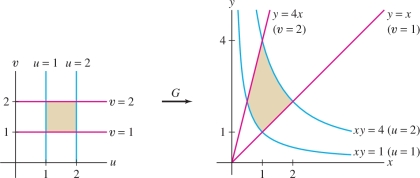
Let \({G}(u,v) = (uv^{-1},uv)\) for \(u>0\), \(v > 0\). Determine the images of:
- (a) The lines \(u=c\) and \(v=c\)
- (b) \([1,2]\times[1,2]\)
Find the inverse map \({G}^{-1}\).
Solution In this map, we have \(x=uv^{-1}\) and \(y=uv\). Thus \begin{equation*} xy = u^2,\qquad \frac{y}x = v^2\tag{3} \end{equation*}
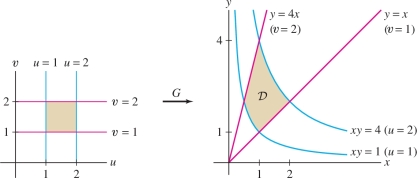
- (a) By the first part of Eq. (3), \(G\) maps a point \((c,v)\) to a point in the \(xy\)-plane with \(xy=c^2\). In other words, \({G}\) maps the vertical line \(u=c\) to the hyperbola \(xy=c^2\). Similarly, by the second part of Eq. (3), the horizontal line \(v=c\) is mapped to the set of points where \(x/y=c^2\), or \(y=c^2x\), which is the line through the origin of slope \(c^2\). See Figure 15.70.
- (b) The image of \([1,2] \times [1,2]\) is the curvilinear rectangle bounded by the four curves that are the images of the lines \(u=1\), \(u=2\), and \(v=1\), \(v=2\). By Eq. (3), this region is defined by the inequalities \[ 1 \le xy \le 4,\qquad 1 \le \frac yx \le 4 \]
The term “curvilinear rectangle” refers to a region bounded on four sides by curves as in Figure 15.70.
To find \({G}^{-1}\), we use Eq. (3) to write \(u=\sqrt{xy}\) and \(v=\sqrt{y/x}\). Therefore, the inverse map is \({G}^{-1}(x,y)=\left(\sqrt{xy}, \sqrt{y/x}\right)\). We take positive square roots because \(u>0\) and \(v > 0\) on the domain we are considering.
923
How Area Changes under a Mapping: The Jacobian Determinant
The Jacobian determinant (or simply the Jacobian) of a map \[ {G}(u,v) = (x(u,v),y(u,v)) \] is the determinant \[ \boxed{ {\textrm{Jac}}({G}) = \left| \begin{array}{cc} \frac{\partial {x}}{\partial u} & \frac{\partial {x}}{\partial v} \\ \frac{\partial {y}}{\partial u} & \frac{\partial {y}}{\partial v} \\ \end{array} \right| = \frac{\partial x}{\partial u}\frac{\partial y}{\partial v}-\frac{\partial x}{\partial v}\frac{\partial y}{\partial u}} \]
The Jacobian \({\textrm{Jac}}({G})\) is also denoted \(\frac{\partial(x,y)}{\partial(u,v)}\). Note that \({\textrm{Jac}}({G})\) is a function of \(u\) and \(v\).
REMINDER
The definition of a \(2\times 2\) determinant is \begin{equation*} \left| \begin{array}{cc} a & b \\ c & d \\ \end{array} \right| = ad-bc\tag{4} \end{equation*}
EXAMPLE 4
Evaluate the Jacobian of \({G}(u,v) = (u^3+v,uv)\) at \((u,v)=(2,1)\).
Solution We have \(x=u^3+v\) and \(y=uv\), so \[ \begin{array}{rl} {\textrm{Jac}}({G})&= \frac{\partial(x,y)}{\partial(u,v)} = \left|\begin{array}{cc} \frac{\partial x}{\partial u} & \frac{\partial x}{\partial v} \\ \frac{\partial y}{\partial u} & \frac{\partial y}{\partial v} \\ \end{array}\right|\\ &= \Big|\begin{array}{cc} 3u^2 & 1 \\ v & u \\ \end{array}\Big| = 3u^3-v \end{array} \]
The value of the Jacobian at \((2,1)\) is \({\textrm{Jac}}({G})(2,1) = 3(2)^3-1 = 23\).
924
The Jacobian tells us how area changes under a map \({G}\). We can see this most directly in the case of a linear map \({G}(u,v)=(Au+Cv,Bu+Dv)\).
THEOREM 1 Jacobian of a Linear Map
The Jacobian of a linear map \[ {G}(u,v)=(Au+Cv,Bu+Dv) \] is constant with value \begin{equation*} {\textrm{Jac}}({G}) = \left| \begin{array}{cc} A& C\\ B & D\\ \end{array} \right| = AD-BC\tag{5} \end{equation*}
Under \({G}\), the area of a region \({\mathcal{D}}\) is multiplied by the factor \(|{\textrm{Jac}}({G})|\); that is, \begin{equation*} \boxed{\textrm{Area}({G}({\mathcal{D}})) = |{\textrm{Jac}}({G})|\textrm{Area}({\mathcal{D}})}\tag{6} \end{equation*}
Proof Eq. (5) is verified by direct calculation: Because \[ x=Au+Cv \quad\text{ and}\quad y=Bu+Dv \] the partial derivatives in the Jacobian are the constants \(A, B, C, D\).
We sketch a proof of Eq. (6). It certainly holds for the unit rectangle \({\mathcal{D}} =[1,0] \times [0,1]\) because \({G}({\mathcal{D}})\) is the parallelogram spanned by the vectors \(\left\langle A,B \right\rangle\) and \(\left\langle C,D\right\rangle\) Figure 15.71 and this parallelogram has area \[ |{\textrm{Jac}}({G})|=|AD-BC| \] by Theorem 3 in Section 12.4. Similarly, we can check directly that Eq. (6) holds for arbitrary parallelograms (see Exercise 48). To verify Eq. (6) for a general domain \({\mathcal{D}}\), we use the fact that \({\mathcal{D}}\) can be approximated as closely as desired by a union of rectangles in a fine grid of lines parallel to the \(u\)- and \(v\)-axes.
We cannot expect Eq. (6) to hold for a nonlinear map. In fact, it would not make sense as stated because the value \({\textrm{Jac}}({G})(P)\) may vary from point to point. However, it is approximately true if the domain \({\mathcal{D}}\) is small and \(P\) is a sample point in \({\mathcal{D}}\): \begin{equation*} \boxed{\textrm{Area}({G}({\mathcal{D}})) \approx |{\textrm{Jac}}({G})(P)|\textrm{Area}({\mathcal{D}})}\tag{7} \end{equation*}
This result may be stated more precisely as the limit relation: \begin{equation*} |{\textrm{Jac}}({G})(P)| = \lim_{|{\mathcal{D}}|\to 0}\, \frac{\textrm{Area}({G}({\mathcal{D}}))}{\textrm{Area}({\mathcal{D}})}\tag{8} \end{equation*}
Here, we write \(|{\mathcal{D}}|\to 0\) to indicate the limit as the diameter of \({\mathcal{D}}\) (the maximum distance between two points in \({\mathcal{D}}\)) tends to zero.
925
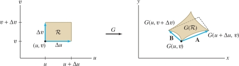
CONCEPTUAL INSIGHT
Although a rigorous proof of Eq. (8) is too technical to include here, we can understand Eq. (7) as an application of linear approximation. Consider a rectangle \({\mathcal{R}}\) with vertex at \(P=(u,v)\) and sides of lengths \(\Delta u\) and \(\Delta v\), assumed to be small as in Figure 15.72. The image \({G}({\mathcal{R}})\) is not a parallelogram, but it is approximated well by the parallelogram spanned by the vectors \({\bf{A}}\) and \({\bf{B}}\) in the figure: \[ \begin{array}{rl} {\bf{A}} &= {G}(u+\Delta u,v) - {G}(u,v)\\&=({x}(u+\Delta u,v)-{x}(u,v),{y}(u+\Delta u,v)-{y}(u,v)) \\ {\bf{B}} &= {G}(u,v+\Delta v) - {G}(u,v)\\ &=({x}(u,v+\Delta v)-{x}(u,v),{y}(u,v+\Delta v)-{y}(u,v)) \end{array} \]
The linear approximation applied to the components of \({G}\) yields \begin{equation*} {\bf{A}} \approx \left\langle \frac{\partial x}{\partial u}\Delta u, \frac{\partial y}{\partial u}\Delta u \right\rangle\tag{9} \end{equation*} \begin{equation*} {\bf{B}} \approx \left\langle \frac{\partial x}{\partial v}\Delta v, \frac{\partial y}{\partial v}\Delta v \right\rangle\tag{10} \end{equation*}
This yields the desired approximation: \[ \begin{array}{rl} \textrm{Area}({G}({\mathcal{R}}))&\approx \left| \det\left( \begin{array}{c} {\bf{A}}\\ {\bf{B}} \\ \end{array} \right)\right| = \left| \det\left( \begin{array}{cc} \frac{\partial x}{\partial u}\Delta u &\frac{\partial y}{\partial u}\Delta u\\ \frac{\partial x}{\partial v}\Delta v &\frac{\partial y}{\partial v}\Delta v \\ \end{array} \right)\right| \\ &= \left|\frac{\partial x}{\partial u}\frac{\partial y}{\partial v}- \frac{\partial y}{\partial u}\frac{\partial x}{\partial v}\right|\, \Delta u\,\Delta v \\ & = |{\textrm{Jac}}({G})(P)|\textrm{Area}({\mathcal{R}}) \end{array} \] since the area of \({\mathcal{R}}\) is \(\Delta u\,\Delta v\).
REMINDER
Equations (9) and (10) use the linear approximations \[ \begin{array}{rl} {x}(u+\Delta u,v)-{x}(u,v)&\approx \frac{\partial x}{\partial u}\Delta u\\ {y}(u+\Delta u ,v)-{y}(u,v)&\approx \frac{\partial y}{\partial u}\Delta u \end{array} \] and \[ \begin{array}{rl} {x}(u,v+\Delta v)-{x}(u,v)&\approx \frac{\partial x}{\partial v}\Delta v\\ {y}(u,v+\Delta v)-{y}(u,v)&\approx \frac{\partial y}{\partial v}\Delta v \end{array} \]
The Change of Variables Formula
Recall the formula for integration in polar coordinates: \begin{equation*} \iint_{{\mathcal{D}}\,} f(x,y)\, dx\,dy = \int_{\theta_1}^{\theta_2}\int_{r_1}^{r_2} f(r\cos\theta,r\sin\theta)\,r\,dr\,d\theta\tag{11} \end{equation*}
Here, \({\mathcal{D}}\) is the polar rectangle consisting of points \((x,y) = (r \cos\theta, r \sin\theta )\) in the \(xy\)-plane (see Figure 15.67 above). The domain of integration on the right is the rectangle \({\mathcal{R}} = [\theta_1, \theta_2]\times [r_1, r_2]\) in the \(r\theta\)-plane. Thus, \({\mathcal{D}}\) is the image of the domain on the right under the polar coordinates map.
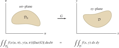
The general Change of Variables Formula has a similar form. Given a map \[ {G}: \quad\underset{\textrm{in }uv\textrm{-plane}}{{\mathcal{D}}_0}\quad\rightarrow\quad \underset{\textrm{in }xy\textrm{-plane}}{{\mathcal{D}}} \] from a domain in the \(uv\)-plane to a domain in the \(xy\)-plane Figure 15.73, our formula expresses an integral over \({\mathcal{D}}\) as an integral over \({\mathcal{D}}_0\). The Jacobian plays the role of the factor \(r\) on the right-hand side of Eq. (11).
REMINDER
\({G}\) is called “one-to-one” if \({G}(P) = {G}(Q)\) only for \(P=Q\).
A few technical assumptions are necessary. First, we assume that \({G}\) is one-to-one, at least on the interior of \({\mathcal{D}}_0\), because we want \({G}\) to cover the target domain \({\mathcal{D}}\) just once. We also assume that \({G}\) is a \(C^1\) map, by which we mean that the component functions \({x}\) and \({y}\) have continuous partial derivatives. Under these conditions, if \(f(x,y)\) is continuous, we have the following result.
926
THEOREM 2 Change of Variables Formula
Let \({G}:{\mathcal{D}}_0\to{\mathcal{D}}\) be a \(C^1\) mapping that is one-to-one on the interior of \({\mathcal{D}}_0\). If \(f(x,y)\) is continuous, then \begin{equation*} \boxed{\iint_{{\mathcal{D}}\,} f(x,y)\,dx\,dy = \iint_{{\mathcal{D}}_0\,} f(x(u,v),y(u,v))\left| \frac{\partial(x,y)}{\partial(u,v)}\right|\,du\,dv}\tag{12} \end{equation*}
Eq. (12) is summarized by the symbolic equality \[ \boxed{dx\,dy=\left|\frac{\partial(x,y)}{\partial(u,v)}\right|\,du\,dv} \] Recall that \(\frac{\partial(x,y)}{\partial(u,v)}\) denotes the Jacobian \({\textrm{Jac}}({G})\).
Proof We sketch the proof. Observe first that Eq. (12) is approximately true if the domains \({\mathcal{D}}_0\) and \({\mathcal{D}}\) are small. Let \(P = {G}(P_0)\) where \(P_0\) is any sample point in \({\mathcal{D}}_0\). Since \(f(x,y)\) is continuous, the approximation recalled in the margin together with Eq. (7) yield \[ \begin{array}{rl} \iint_{{\mathcal{D}}\,} f(x,y)\,dx\,dy &\approx f(P)\textrm{Area}({\mathcal{D}}) \\ &\approx f({G}(P_0))\,|{\textrm{Jac}}({G})(P_0)|\,\textrm{Area}({\mathcal{D}}_0)\\ & \approx \iint_{{\mathcal{D}}_0\,} f({G}(u,v))\,|{\textrm{Jac}}({G})(u,v)|\,du\,dv \end{array} \]
REMINDER
If \({\mathcal{D}}\) is a domain of small diameter, \(P\in{\mathcal{D}}\) is a sample point, and \(f(x,y)\) is continuous, then (see Section 15.2) \[ \iint_{{\mathcal{D}}\,} f(x,y)\,dx\,dy \approx f(P)\textrm{Area}({\mathcal{D}}) \]
If \({\mathcal{D}}\) is not small, divide it into small subdomains \(D_j={G}({\mathcal{D}}_{0j})\) (Figure 15.74 shows a rectangle divided into smaller rectangles), apply the approximation to each subdomain, and sum: \[ \begin{array}{rl} \iint_{{\mathcal{D}}\,} f(x,y)\,dx\,dy &= \sum_{j} \iint_{{\mathcal{D}}_j\,} f(x,y)\,dx\,dy \\ &\approx \sum_{j} \iint_{{\mathcal{D}}_{0j}\,} f({G}(u,v)))\,|{\textrm{Jac}}({G})(u,v)|\,du\,dv \\ &=\iint_{{\mathcal{D}}_0\,} f({G}(u,v))\,|{\textrm{Jac}}({G})(u,v)|\,du\,dv \end{array} \]
Careful estimates show that the error tends to zero as the maximum of the diameters of the subdomains \({\mathcal{D}}_j\) tends to zero. This yields the Change of Variables Formula.
927
EXAMPLE 5 Polar Coordinates Revisited
Use the Change of Variables Formula to derive the formula for integration in polar coordinates.
Solution The Jacobian of the polar coordinate map \({G}(r,\theta)=(r\cos\theta, r\sin\theta)\) is \[ {\textrm{Jac}}({G})=\left| \begin{array}{cc} \displaystyle\frac{\partial x}{\partial r} & \displaystyle\frac{\partial x}{\partial \theta} \\ \displaystyle\frac{\partial y}{\partial r}& \displaystyle\frac{\partial y}{\partial \theta} \\ \end{array} \right| = \left| \begin{array}{cc} \cos\theta & -r\sin\theta \\ \sin\theta& r\cos\theta \\ \end{array} \right|=r(\cos^2\theta+\sin^2\theta)=r \]
Let \({\mathcal{D}} = G({\mathcal{R}})\) be the image under the polar coordinates map \(G\) of the rectangle \({\mathcal{R}}\) defined by \(r_0\le r \le r_1\), \(\theta_0 \le \theta \le \theta_1\) (see Figure 15.75). Then Eq. (12) yields the expected formula for polar coordinates: \begin{equation*} \iint_{{\mathcal{D}}\,} f(x,y)\,dx\,dy = \int_{\theta_0}^{\theta_1}\int_{r_0}^{r_1} f(r\cos\theta,r\sin\theta)\,r\,dr\,d\theta\tag{13} \end{equation*}
Assumptions Matter In the Change of Variables Formula, we assume that \({G}\) is one-to-one on the interior but not necessarily on the boundary of the domain. Thus, we can apply Eq. (12) to the polar coordinates map \({G}\) on the rectangle \({\mathcal{D}}_0=[0,1]\times [0,2\pi]\). In this case, \({G}\) is one-to-one on the interior but not on the boundary of \({\mathcal{D}}_0\) since \({G}(0,\theta) = (0,0)\) for all \(\theta\) and \({G}(r,0)={G}(r,2\pi)\) for all \(r\). On the other hand, Eq. (12) cannot be applied to \({G}\) on the rectangle \([0,1]\times [0,4\pi]\) because it is not one-to-one on the interior.
EXAMPLE 6
Use the Change of Variables Formula to calculate \(\iint_{{\mathcal{P}}\,} e^{4x-y}\,dx\,dy\), where \({\mathcal{P}}\) is the parallelogram spanned by the vectors \(\left\langle 4,1\right\rangle\), \(\left\langle 3,3\right\rangle\) in Figure 15.75.
Recall that the linear map \[ {G}(u,v)=(Au+Cv,Bu+Dv) \] satisfies \[ {G}(1,0)=(A,B),\quad {G}(0,1)=(C,D) \]
Solution
Step 1. Define a map.
We can convert our double integral to an integral over the unit square \({\mathcal{R}}=[0,1]\times[0,1]\) if we can find a map that sends \({\mathcal{R}}\) to \({\mathcal{P}}\). The following linear map does the job: \[ \begin{array}{rl} {G}(u,v)&=(4u+3v,u+3v) \end{array} \]
Indeed, \({G}(1,0)=(4,1)\) and \({G}(0,1)=(3,3)\), so it maps \({\mathcal{R}}\) to \({\mathcal{P}}\) because linear maps map parallelograms to parallelograms.
Step 2. Compute the Jacobian.
\[ {\textrm{Jac}}({G}) = \left| \begin{array}{cc} \frac{\partial x}{\partial u} & \frac{\partial x}{\partial v} \\ \frac{\partial y}{\partial u} & \frac{\partial y}{\partial v} \\ \end{array} \right| = \left| \begin{array}{cc} 4 & 3 \\ 1 & 3 \end{array} \right| = 9 \]
928
Step 3. Express \(f(x,y)\) in terms of the new variables.
Since \(x = 4u+3v\) and \(y=u+3v\), we have \[ e^{4x-y} = e^{4(4u+3v)-(u+3v)} = e^{15u+9v} \]
Step 4. Apply the Change of Variables Formula.
The Change of Variables Formula tells us that \(dx\,dy = 9\,du\,dv\): \[ \begin{array}{rl} \iint_{{\mathcal{P}}\,} e^{4x-y}\,dx\,dy &=\iint_{\!{\mathcal{R}}\,} e^{15u+9v}\,|{\textrm{Jac}}({G})|\,du\,dv = \int_0^1\int_0^1 e^{15u+9v}\,(9\,du\,dv)\\ &=9\left(\int_0^1\,e^{15u}\,du\right)\left(\int_0^1 e^{9v} \,dv\right) =\frac1{15}(e^{15}-1)(e^9-1) \end{array} \]
EXAMPLE 7
Use the Change of Variables Formula to compute \[ \iint_{{\mathcal{D}}\,}(x^2+y^2)\,dx\,dy \] where \({\mathcal{D}}\) is the domain \(1\le xy\le 4\), \(1\le y/x \le 4\) Figure 15.76.
Solution In Example 3, we studied the map \({G}(u,v) = (uv^{-1}, uv)\), which can be written \[ x=uv^{-1} ,\qquad y=uv \]
We showed Figure 15.76 that \({G}\) maps the rectangle \({\mathcal{D}}_0=[1,2] \times [1,2]\) to our domain \({\mathcal{D}}\). Indeed, because \(xy=u^2\) and \(xy^{-1} = v^2\), the two conditions \(1\le xy\le 4\) and \(1\le y/x \le 4\) that define \({\mathcal{D}}\) become \(1\le u\le 2\) and \(1\le v \le 2\).
The Jacobian is \[ {\textrm{Jac}}({G}) = \frac{\partial(x,y)}{\partial(u,v)} = \left| \begin{array}{cc} \frac{\partial x}{\partial u} & \frac{\partial x}{\partial v} \\ \frac{\partial y}{\partial u} & \frac{\partial y}{\partial v} \\ \end{array} \right| = \left| \begin{array}{cc} v^{-1} & -uv^{-2} \\ v & u \\ \end{array} \right| = \frac{2u}v \]
To apply the Change of Variables Formula, we write \(f(x,y)\) in terms of \(u\) and \(v\): \[ f(x,y)=x^2+y^2 = \left(\frac{u}v\right)^2 + (uv)^2 = u^2(v^{-2}+v^2) \]
By the Change of Variables Formula, \[ \begin{array}{rl} \iint_{{\mathcal{D}}\,}(x^2+y^2)\,dx\,dy &= \iint_{{\mathcal{D}}_0\,}\,u^2(v^{-2}+v^2)\left|\frac{2u}v\right|\,du\,dv\\ &= 2 \int_{v=1}^2\int_{u=1}^2 u^3(v^{-3}+v)\,du\,dv\\ &= 2\left( \int_{u=1}^2u^3\,du\right)\left(\int_{v=1}^2 (v^{-3}+v) \,dv\right)\\ &= 2\left(\frac14u^4\bigg|_1^2\right)\left(-\frac12v^{-2}+\frac12v^2\bigg|_1^2\right) = \frac{225}{16} \end{array} \]
929
Keep in mind that the Change of Variables Formula turns an \(xy\)-integral into a \(uv\)-integral, but the map \(G\) goes from the \(uv\)-domain to the \(xy\)-domain. Sometimes, it is easier to find a map \(F\) going in the wrong direction, from the \(xy\)-domain to the \(uv\)-domain. The desired map \(G\) is then the inverse \(G =F^{-1}\). The next example shows that in some cases, we can evaluate the integral without solving for \({G}\). The key fact is that the Jacobian of \(F\) is the reciprocal of \({\textrm{Jac}}({G})\) (see Exercises 49–51): \begin{equation*} \boxed{{\textrm{Jac}}(G) = {\textrm{Jac}}(F)^{-1}\qquad\textrm{where }F ={G}^{-1}}\tag{14} \end{equation*}
Eq. (14) can be written in the suggestive form \[ \boxed{ \frac{\partial(x,y)}{\partial(u,v)} = \left(\frac{\partial(u,v)}{\partial(x,y)}\right)^{-1} } \]
EXAMPLE 8 Using the Inverse Map
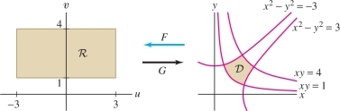
Integrate \(f(x,y) = xy(x^2+y^2)\) over \[ {\mathcal{D}}: -3\le x^2-y^2\le 3,\quad 1\le xy\le 4 \]
Solution There is a simple map \(F\) that goes in the wrong direction. Let \(u=x^2-y^2\) and \(v=xy\). Then our domain is defined by the inequalities \(-3\le u\le 3\) and \(1\le v \le 4\), and we can define a map from \({\mathcal{D}}\) to the rectangle \({\mathcal{R}} = [-3,3]\times [1,4]\) in the \(uv\)-plane Figure 15.77: \[ \begin{array}{rl} F: {\mathcal{D}} &\to {\mathcal{R}} \\ (x,y) &\to (x^2-y^2,xy) \end{array} \]
To convert the integral over \({\mathcal{D}}\) into an integral over the rectangle \({\mathcal{R}}\), we have to apply the Change of Variables Formula to the inverse mapping: \[ {G} = F^{-1}:{\mathcal{R}} \to {\mathcal{D}} \]
We will see that it is not necessary to find \({G}\) explicitly. Since \(u=x^2-y^2\) and \(v=xy\), the Jacobian of \(F\) is \[ \begin{array}{rl} {\textrm{Jac}}(F)& = \left| \begin{array}{cc} \displaystyle\frac{\partial u}{\partial x} & \displaystyle\frac{\partial u}{\partial y} \\ \displaystyle\frac{\partial v}{\partial x} & \displaystyle\frac{\partial v}{\partial y} \\ \end{array} \right| = \left| \begin{array}{cc} 2x & -2y \\ y & x \\ \end{array} \right| = 2(x^2+y^2) \end{array} \]
930
By Eq. (14), \[ {\textrm{Jac}}({G}) = {\textrm{Jac}}(F)^{-1} = \frac1{2(x^2+y^2)} \]
Normally, the next step would be to express \(f(x,y)\) in terms of \(u\) and \(v\). We can avoid doing this in our case by observing that the Jacobian cancels with one factor of \(f(x,y)\): \[ \begin{array}{rl} \iint_{{\mathcal{D}}\,} xy(x^2+y^2) \,dx\,dy &=\iint_{{\mathcal{R}}\,} f(x(u,v), y(u,v))\,\left|{\textrm{Jac}}({G})\right|\,du\,dv \\ &= \iint_{{\mathcal{R}}\,} xy(x^2+y^2) \frac{1}{2(x^2+y^2)}\,du\,dv \\ &= \frac12 \iint_{{\mathcal{R}}\,} xy\,du\,dv \\&= \frac12 \iint_{{\mathcal{R}}\,} v\,du\,dv\qquad(\textrm{because }v=xy)\\ &= \frac12\int_{-3}^3 \int_1^4v\,dv\,du = \frac12 (6)\left(\frac124^2-\frac121^2\right) = \frac{45}2 \end{array} \]
Change of Variables in Three Variables
The Change of Variables Formula has the same form in three (or more) variables as in two variables. Let \[ {G}: {\mathcal{W}}_0\to {\mathcal{W}} \] be a mapping from a three-dimensional region \({\mathcal{W}}_0\) in \((u,v,w)\)-space to a region \({\mathcal{W}}\) in \((x,y,z)\)-space, say, \[ x = x(u,v,w),\qquad y = y(u,v,w),\qquad z = z(u,v,w) \]
REMINDER
\(3\times 3\)-determinants are defined in Eq. (2) of Section 12.4.
The Jacobian \({\textrm{Jac}}({G})\) is the \(3\times 3\) determinant: \begin{equation*} {\textrm{Jac}}({G}) = \displaystyle\frac{\partial (x,y,z)}{\partial (u,v,w)} = \left|\begin{array}{ccc} \displaystyle\frac{\partial x}{\partial u} & \displaystyle\frac{\partial x}{\partial v} &\displaystyle \frac{\partial x}{\partial w} \\ \displaystyle\frac{\partial y}{\partial u} & \displaystyle\frac{\partial y}{\partial v} &\displaystyle \frac{\partial y}{\partial w} \\ \displaystyle\frac{\partial z}{\partial u} & \displaystyle\frac{\partial z}{\partial v} &\displaystyle \frac{\partial z}{\partial w} \\ \end{array} \right|\tag{15} \end{equation*}
The Change of Variables Formula states \[ \boxed{dx\,dy\,dz = \left| \frac{\partial(x,y,z)}{\partial(u,v,w)}\right|\,du\,dv\,dw} \]
More precisely, if \({G}\) is \(C^1\) and one-to-one on the interior of \({\mathcal{W}}_0\), and if \(f\) is continuous, then \begin{equation*} \begin{array}{rcl} &&\iiint_{{\mathcal{W}}\,} f(x,y,z)\,dx\,dy\,dz \\ &&\qquad = \iiint_{{\mathcal{W}}_0\,} f(x(u,v,w),y(u,v,w),z(u,v,w)) \left|\frac{\partial(x,y,z)}{\partial(u,v,w)}\right|\,du\,dv\,dw \end{array}\tag{16} \end{equation*}
931
In Exercises 42 and 43, you are asked to use the general Change of Variables Formula to derive the formulas for integration in cylindrical and spherical coordinates developed in Section 15.4.
15.6.1 Summary
- Let \({G}(u,v)=({x}(u,v), {y}(u,v))\) be a mapping. We write \(x={x}(u,v)\) or \(x=x(u,v)\) and, similarly, \(y={y}(u,v)\) or \(y=y(u,v)\). The Jacobian of \({G}\) is the determinant \[ {\textrm{Jac}}({G}) = \frac{\partial(x,y)}{\partial(u,v)} = \left| \begin{array}{cc} \displaystyle\frac{\partial x}{\partial u} & \displaystyle\frac{\partial x}{\partial v}\\ \displaystyle\frac{\partial y}{\partial u} & \displaystyle\frac{\partial y}{\partial v} \\ \end{array} \right| \]
- \({\textrm{Jac}}(G) = {\textrm{Jac}}(F)^{-1}\) where \(F = G^{-1}\).
- Change of Variables Formula: If \({G}:{\mathcal{D}}_0\to{\mathcal{D}}\) is \(C^1\) and one-to-one on the interior of \({\mathcal{D}}_0\), and if \(f\) is continuous, then \[ \iint_{{\mathcal{D}}\,} f(x,y)\,dx\,dy = \iint_{{\mathcal{D}}_0\,} f(x(u,v),y(u,v)) \left|\frac{\partial(x,y)}{\partial(u,v)}\right|\,du\,dv \]
- The Change of Variables Formula is written symbolically in two and three variables as \[ dx\,dy =\left|\frac{\partial(x,y)}{\partial(u,v)}\right|\,du\,dv, \qquad dx\,dy\,dz = \left| \frac{\partial(x,y,z)}{\partial(u,v,w)}\right|\,du\,dv\,dw \]