16.5 Surface Integrals of Vector Fields
The last integrals we will consider are surface integrals of vector fields. These integrals represent flux or rates of flow through a surface. One example is the flux of molecules across a cell membrane (number of molecules per unit time).
The word flux is derived from the Latin word fluere, which means “to flow.”
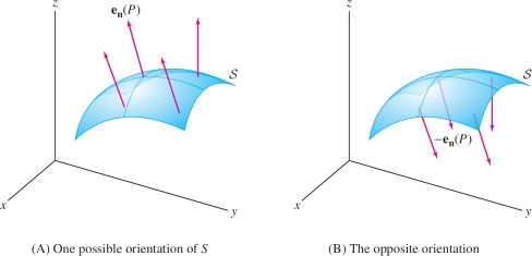
Because flux through a surface goes from one side of the surface to the other, we need to specify a positive direction of flow. This is done by means of an orientation, which is a choice of unit normal vector \({\bf{e}}_{{\bf{n}}}(P)\) at each point \(P\) of \({\mathcal{S}}\), chosen in a continuously varying manner (Figure 16.53). There are two normal directions at each point, so the orientation serves to specify one of the two “sides” of the surface in a consistent manner. The unit vectors \(-{\bf{e}}_{{\bf{n}}}(P)\) define the opposite orientation. For example, if \({\bf{e}}_{{\bf{n}}}\) are outward-pointing unit normal vectors on a sphere, then a flow from the inside of the sphere to the outside is a positive flux.
990
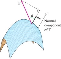
The normal component of a vector field \({\bf{F}}\) at a point \(P\) on an oriented surface \({\mathcal{S}}\) is the dot product \[ \boxed{\textrm{Normal component at } P = {\bf{F}}(P){\cdot}{\bf{e}}_{{\bf{n}}}(P) =\left \| {{\bf{F}}(P)} \right \|\cos\theta} \] where \(\theta\) is the angle between \({\bf{F}}(P)\) and \({\bf{e}}_{{\bf{n}}}(P)\) (Figure 16.54). Often, we write \({\bf{e}}_{{\bf{n}}}\) instead of \({\bf{e}}_{{\bf{n}}}(P)\), but it is understood that \({\bf{e}}_{{\bf{n}}}\) varies from point to point on the surface. The vector surface integral, denoted \(\iint_{{\mathcal{S}}\,}{\bf{F}}{\cdot} d{\bf{S}}\), is defined as the integral of the normal component: \[ \boxed{\textrm{Vector surface integral:}\quad \iint_{{\mathcal{S}}\,}{\bf{F}}{\cdot} d{\bf{S}} = \iint_{{\mathcal{S}}\,}({\bf{F}}{\cdot}{\bf{e}}_{{\bf{n}}})\,dS } \]
This quantity is also called the flux of \({\bf{F}}\) across or through \({\mathcal{S}}\).
An oriented parametrization \({G}(u,v)\) is a regular parametrization (meaning that \({\bf{n}}(u,v)\) is nonzero for all \(u,v\)) whose unit normal vector defines the orientation: \[ {\bf{e}}_{{\bf{n}}} = {\bf{e}}_{{\bf{n}}}(u,v) = \frac{{\bf{n}}(u,v)}{\left \| {{\bf{n}}(u,v)} \right \|} \]
REMINDER
Formula for a scalar surface integral in terms of an oriented parametrization: \begin{equation*} \begin{array}{l} \iint_{{\mathcal{S}}\,}f(x,y,z)\, dS\\ = \iint f({G}(u,v))\left \| {{\bf{n}}(u,v)} \right \| \,du\,dv \end{array}\tag{1} \end{equation*}
Applying Eq. (1) in the margin to \({\bf{F}}{\cdot}{\bf{e}}_n\), we obtain \begin{equation*} \begin{array}{rl} \iint_{{\mathcal{S}}\,}{\bf{F}}{\cdot} d{\bf{S}} & = \iint_{{\mathcal{D}}\,}({\bf{F}}{\cdot}{\bf{e}}_{{\bf{n}}})\left \| {{\bf{n}}(u,v)} \right \|\,du\,dv\\ & = \iint_{{\mathcal{D}}\,}{\bf{F}}({G}(u,v)){\cdot}\left(\frac{{\bf{n}}(u,v)}{\left \| {{\bf{n}}(u,v)} \right \|}\right) \left \| {{\bf{n}}(u,v)} \right \|\,du\,dv\\ & = \iint_{{\mathcal{D}}\,} {\bf{F}}({G}(u,v)){\cdot} {\bf{n}}(u,v) \,du\,dv \end{array}\tag{2} \end{equation*}
This formula remains valid even if \({\bf{n}}(u,v)\) is zero at points on the boundary of the parameter domain \({\mathcal{D}}\). If we reverse the orientation of \({\mathcal{S}}\) in a vector surface integral, \({\bf{n}}(u,v)\) is replaced by \(-{\bf{n}}(u,v)\) and the integral changes sign.
We can think of \(d{\bf{S}}\) as a “vector surface element” that is related to a parametrization by the symbolic equation \[ \boxed{d{\bf{S}} = {\bf{n}}(u,v)\,du\,dv} \]
991
THEOREM 1 Vector Surface Integral
Let \({G}(u,v)\) be an oriented parametrization of an oriented surface \({\mathcal{S}}\) with parameter domain \({\mathcal{D}}\). Assume that \({G}\) is one-to-one and regular, except possibly at points on the boundary of \({\mathcal{D}}\). Then \begin{equation*} \boxed{ \iint_{{\mathcal{S}}\,}{\bf{F}}{\cdot} d{\bf{S}} = \iint_{{\mathcal{D}}\,} {\bf{F}}({G}(u,v)){\cdot} {\bf{n}}(u,v) \,du\,dv}\tag{3} \end{equation*}
If the orientation of \({\mathcal{S}}\) is reversed, the surface integral changes sign.
EXAMPLE 1
Calculate \(\iint_{{\mathcal{S}}\,}{\bf{F}}{\cdot}\,d{\bf{S}}\), where \({\bf{F}} = \left\langle 0,0,x \right\rangle \) and \({\mathcal{S}}\) is the surface with parametrization \({G}(u,v) = (u^2, v, u^3 - v^2)\) for \( 0\le u\le 1,\,\, 0\le v\le 1\) and oriented by upward-pointing normal vectors.
Solution
Step 1. Compute the tangent and normal vectors.
\[ \begin{array}{rl} {\bf{T}}_u &= \big\langle 2u,0,3u^2\big\rangle,\qquad T_v = \left\langle 0,1,-2v\right\rangle\\ {\bf{n}}(u,v) &= {\bf{T}}_u{\times} {\bf{T}}_v = \left| \begin{array}{ccc} {\bf{i}} & {\bf{j}} & {\bf{k}}\\ 2u & 0 & 3u^2\\ 0 & 1 & -2v \end{array} \right| \\ &= -3u^2{\bf{i}} + 4uv{\bf{j}} + 2u{\bf{k}} = \big\langle-3u^2, 4uv, 2u\big\rangle \end{array} \]
The \(z\)-component of \({\bf{n}}\) is positive on the domain \(0\le u\le 1\), so \({\bf{n}}\) is the upward-pointing normal (Figure 16.55).
Step 2. Evaluate \({\bf{F}}{\cdot} {\bf{n}}\).
Write \({\bf{F}}\) in terms of the parameters \(u\) and \(v\). Since \(x= u^2\), \[ {\bf{F}}({G}(u,v)) = \left\langle 0,0,x \right\rangle = \big\langle 0,0,u^2\big\rangle \] and \[ {\bf{F}}({G}(u,v)){\cdot} {\bf{n}}(u,v) = \big\langle 0,0,u^2\big\rangle {\cdot}\big\langle-3u^2, 4uv, 2u\big\rangle = 2u^3 \]
Step 3. Evaluate the surface integral.
The parameter domain is \(0\le u\le1\), \(0\le v\le 1\), so \[ \begin{array}{rl} \iint_{{\mathcal{S}}\,} {\bf{F}}{\cdot} d{\bf{S}} &= \int_{u=0}^1\int_{v=0}^1 {\bf{F}}({G}(u,v)){\cdot}{\bf{n}}(u,v)\,dv\,du \\ &= \int_{u=0}^1\int_{v=0}^1 2u^3\,dv\,du = \int_{u=0}^1 2u^3 \,du =\frac12 \end{array} \]
EXAMPLE 2 Integral over a Hemisphere
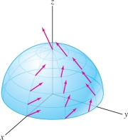
Calculate the flux of \({\bf{F}} = \left\langle z, x, 1 \right\rangle \) across the upper hemisphere \({\mathcal{S}}\) of the sphere \(x^2+y^2+z^2=1\), oriented with outward-pointing normal vectors (Figure 16.56).
Solution Parametrize the hemisphere by spherical coordinates: \[ {G}(\theta,\phi) = (\cos\theta\sin\phi, \sin\theta\sin\phi,\cos\phi),\qquad 0\le\phi\le \frac{\pi}2, \quad 0 \le \theta< 2\pi \]
Step 1. Compute the normal vector.
According to Eq.(2) in Section 16.4, the outward-pointing normal vector is \[ {\bf{n}} = {\bf{T}}_\phi{\times} {\bf{T}}_\theta = \sin\phi\big\langle\cos\theta\sin \phi, \sin\theta\sin \phi,\cos\phi\big\rangle \]
992
Step 2. Evaluate \({\bf{F}}{\cdot} {\bf{n}}\).
\[ \begin{array}{rcl} {\bf{F}}({G}(\theta,\phi)) &=& \left\langle z, x, 1\right\rangle = \big\langle\cos \phi, \cos\theta\sin \phi,1 \big\rangle\\ {\bf{F}}({G}(\theta,\phi))\cdot {\bf{n}}(\theta,\phi) &=& \big\langle \cos \phi, \cos\theta\sin \phi,1 \big\rangle {\cdot} \big\langle \cos\theta\sin^2\phi, \sin\theta\sin^2\phi,\cos\phi\sin\phi\big\rangle \\ &=&\cos\theta\sin^2\phi\cos \phi+ \cos\theta\sin\theta \sin^3\phi +\cos\phi\sin\phi \end{array} \]
Step 3. Evaluate the surface integral.
\[ \begin{array}{rl} \iint_{{\mathcal{S}}\,}{\bf{F}}{\cdot} d{\bf{S}} &= \int_{\phi=0}^{\pi/2} \int_{\theta=0}^{2\pi} {\bf{F}}({G}(\theta,\phi)){\cdot} {\bf{n}}(\theta,\phi)\,d\theta\,d\phi\\ & = \int_{\phi=0}^{\pi/2} \int_{\theta=0}^{2\pi} ( \underbrace{\cos\theta\sin^2\phi\cos \phi+ \cos\theta\sin\theta \sin^3\phi}_{\textrm{Integral over }\theta \textrm{ is zero}} +\cos\phi\sin\phi)\,d\theta\,d\phi \end{array} \]
The integrals of \(\cos\theta\) and \(\cos\theta\sin\theta\) over \([0, 2\pi]\) are both zero, so we are left with \[ \int_{\phi=0}^{\pi/2} \int_{\theta=0}^{2\pi}\cos\phi\sin\phi \,d\theta\,d\phi = 2\pi \int_{\phi=0}^{\pi/2} \cos\phi\sin\phi \, d\phi = -2\pi \frac{\cos^2\phi}2\bigg|_0^{\pi/2} = \pi \]
EXAMPLE 3 Surface Integral over a Graph
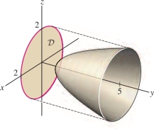
Calculate the flux of \({\bf{F}} = x^2{\bf{j}}\) through the surface \({\mathcal{S}}\) defined by \(y=1+x^2+z^2\) for \(1\le y \le 5\). Orient \({\mathcal{S}}\) with normal pointing in the negative \(y\)-direction.
Solution This surface is the graph of the function \(y=1+x^2+z^2\), where \(x\) and \(z\) are the independent variables (Figure 16.57).
Step 1. Find a parametrization.
It is convenient to use \(x\) and \(z\) because \(y\) is given explicitly as a function of \(x\) and \(z\). Thus we define \[ {G}(x,z)=(x,1+x^2+z^2,z) \]
What is the parameter domain? The condition \(1\le y\le 5\) is equivalent to \(1\le 1+x^2+z^2 \le 5\) or \(0\le x^2+z^2 \le 4\). Therefore, the parameter domain is the disk of radius \(2\) in the \(xz\)-plane—that is, \({\mathcal{D}}=\{(x,z): x^2+z^2\le 4\}\).
Because the parameter domain is a disk, it makes sense to use the polar variables \(r\) and \(\theta\) in the \(xz\)-plane. In other words, we write \(x=r\cos\theta\), \(z=r\sin\theta\). Then \[ y = 1+x^2+z^2=1+r^2 \] \[ {G}(r,\theta)=(r\cos\theta,1+r^2,r\sin\theta),\quad 0\le\theta\le 2\pi,\quad 0\le r\le 2 \]
Step 2. Compute the tangent and normal vectors.
\[ \begin{array}{rl} {\bf{T}}_r &= \left\langle \cos\theta,2r,\sin\theta\right\rangle,\qquad {\bf{T}}_\theta = \left\langle -r\sin\theta, 0, r\cos\theta\right\rangle\\ {\bf{n}} &= {\bf{T}}_r{\times} {\bf{T}}_\theta = \left| \begin{array}{ccc} {\bf{i}} & {\bf{j}} & {\bf{k}}\\ \cos\theta&2r&\sin\theta\\ -r\sin\theta& 0& r\cos\theta \end{array} \right| = 2r^2\cos\theta{\bf{i}}-r{\bf{j}}+2r^2\sin\theta{\bf{k}} \end{array} \]
The coefficient of \({\bf{j}}\) is \(-r\). Because it is negative, \({\bf{n}}\) points in the negative \(y\)-direction, as required.
993
CAUTION
In Step 3, we integrate \({\bf{F}}{\cdot}{\bf{n}}\) with respect to \(dr\,d\theta\), and not \(r\,dr\,d\theta\). The factor of \(r\) in \(r\,dr\,d\theta\) is a Jacobian factor that we add only when changing variables in a double integral. In surface integrals, the Jacobian factor is incorporated into the magnitude of \({\bf{n}}\) (recall that \(\left \| {\bf{n}} \right \|\) is the area “distortion factor”).
Step 3. Evaluate \({\bf{F}}{\cdot} {\bf{n}}\).
\[ \begin{array}{rl} {\bf{F}}({G}(r,\theta)) &= x^2{\bf{j}} = r^2\cos^2\theta{\bf{j}} = \big\langle 0, r^2\cos^2\theta, 0\big\rangle\\ {\bf{F}}({G}(r,\theta)){\cdot} {\bf{n}} &= \big\langle 0, r^2\cos^2\theta, 0\big\rangle{\cdot} \left\langle 2r^2\cos\theta,-r,2r^2\sin\theta\right\rangle = -r^3 \cos^2\theta\\ \iint_{{\mathcal{S}}\,}{\bf{F}}{\cdot}\, d{\bf{S}} &= \iint_{{\mathcal{D}}\,} {\bf{F}}({G}(r,\theta)){\cdot} {\bf{n}}\,dr\,d\theta = \int_0^{2\pi}\int_0^2\,\,( -r^3 \cos^2\theta)\,dr\,d\theta\\ &= -\left(\int_0^{2\pi}\cos^2\theta\,d\theta\right) \left(\int_0^2\,\, r^3 \,dr\right)\\ &= -(\pi)\left(\frac{2^4}4\right) = -4\pi \end{array} \]
CONCEPTUAL INSIGHT
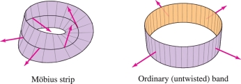
Since a vector surface integral depends on the orientation of the surface, this integral is defined only for surfaces that have two sides. However, some surfaces, such as the Möbius strip (discovered in 1858 independently by August Möbius and Johann Listing), cannot be oriented because they are one-sided. You can construct a Möbius strip \(M\) with a rectangular strip of paper: Join the two ends of the strip together with a \(180^\circ\) twist. Unlike an ordinary two-sided strip, the Möbius strip \(M\) has only one side, and it is impossible to specify an outward direction in a consistent manner (Figure 16.58). If you choose a unit normal vector at a point \(P\) and carry that unit vector continuously around \(M\), when you return to \(P\), the vector will point in the opposite direction. Therefore, we cannot integrate a vector field over a Möbius strip, and it is not meaningful to speak of the “flux” across \(M\). On the other hand, it is possible to integrate a scalar function. For example, the integral of mass density would equal the total mass of the Möbius strip.
Fluid Flux
Imagine dipping a net into a stream of flowing water (Figure 16.59). The flow rate is the volume of water that flows through the net per unit time.
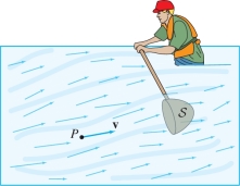
To compute the flow rate, let \({\bf{v}}\) be the velocity vector field. At each point \(P\), \({\bf{v}}(P)\) is velocity vector of the fluid particle located at the point \(P\). We claim that the flow rate through a surface \({\mathcal{S}}\) is equal to the surface integral of \({\bf{v}}\) over \({\mathcal{S}}\).
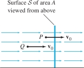
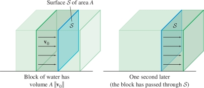
To explain why, suppose first that \({\mathcal{S}}\) is a rectangle of area \(A\) and that \({\bf{v}}\) is a constant vector field with value \({\bf{v}}_0\) perpendicular to the rectangle. The particles travel at speed \(\left \| {{\bf{v}}_0} \right \|\), say in meters per second, so a given particle flows through \({\mathcal{S}}\) within a one-second time interval if its distance to \({\mathcal{S}}\) is at most \(\left \| {{\bf{v}}_0} \right \|\) meters—in other words, if its velocity vector passes through \({\mathcal{S}}\) (see Figure 16.60). Thus the block of fluid passing through \({\mathcal{S}}\) in a one-second interval is a box of volume \(\left \| {{\bf{v}}_0} \right \|A\) (Figure 16.61), and \[ \textrm{Flow rate} = (\textrm{velocity})(\textrm{area}) = \left \| {{\bf{v}}_0} \right \|A \]
994
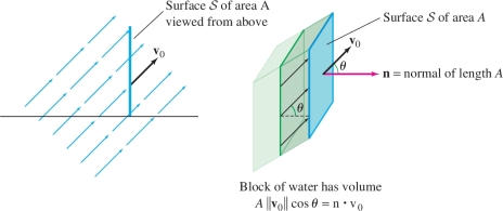
If the fluid flows at an angle \(\theta\) relative to \({\mathcal{S}}\), then the block of water is a parallelepiped (rather than a box) of volume \(A\left \| {{\bf{v}}_0} \right \|\cos\theta\) (Figure 16.62). If \({\bf{n}}\) is a vector normal to \({\mathcal{S}}\) of length equal to the area \(A\), then we can write the flow rate as a dot product: \[ \textrm{Flow rate} = A\left \| {{\bf{v}}_0} \right \|\cos\theta = {\bf{v}}_0{\cdot}{\bf{n}} \]
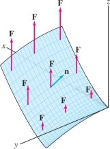
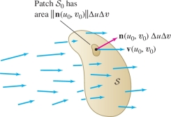
In the general case, the velocity field \({\bf{v}}\) is not constant, and the surface \({\mathcal{S}}\) may be curved. To compute the flow rate, we choose a parametrization \({G}(u,v)\) and we consider a small rectangle of size \(\Delta u \times \Delta v\) that is mapped by \({G}\) to a small patch \({\mathcal{S}}_0\) of \({\mathcal{S}}\) (Figure 16.63). For any sample point \({G}(u_0,v_0)\) in \({\mathcal{S}}_0\), the vector \({\bf{n}}(u_0,v_0)\,\Delta u\,\Delta v\) is a normal vector of length approximately equal to the area of \({\mathcal{S}}_0\) [Eq. (3) in Section 16.4]. This patch is nearly rectangular, so we have the approximation \[ \textrm{Flow rate through }{\mathcal{S}}_0\approx {\bf{v}}(u_0,v_0){\cdot}{\bf{n}}(u_0,v_0)\,\Delta u\,\Delta v \]
The total flow per second is the sum of the flows through the small patches. As usual, the limit of the sums as \(\Delta u\) and \(\Delta v\) tend to zero is the integral of \({\bf{v}}(u,v){\cdot} {\bf{n}}(u,v)\), which is the surface integral of \({\bf{v}}\) over \({\mathcal{S}}\).
Flow Rate through a Surface
For a fluid with velocity vector field \({\bf{v}}\), \begin{equation*} \boxed{\textrm{Flow rate across the }{\mathcal{S}}\textrm{ (volume per unit time)} = \iint_{{\mathcal{S}}\,} {\bf{v}}{\cdot}\,d{\bf{S}}}\tag{4} \end{equation*}
995
EXAMPLE 4
Let \({\bf{v}} = \left\langle x^2+y^2,0,z^2\right\rangle\) be the velocity field (in centimeters per second) of a fluid in \({\bf{R}}^3\). Compute the flow rate through the upper hemisphere \({\mathcal{S}}\) of the unit sphere centered at the origin.
Solution We use spherical coordinates: \[ x = \cos\theta\sin\phi,\qquad y = \sin\theta\sin\phi,\qquad z = \cos\phi \]
The upper hemisphere corresponds to the ranges \(0 \le \phi \le \frac{\pi}2\) and \(0 \le \theta \le 2\pi\). By Eq.(2) in Section 16.4, the upward-pointing normal is \[ {\bf{n}} = {\bf{T}}_{\phi} {\times} {\bf{T}}_{\theta} = \sin\phi\big\langle \cos\theta\sin\phi, \sin\theta\sin\phi, \cos\phi\big\rangle \]
We have \(x^2+y^2 =\sin^2\phi\), so \[ \begin{array}{rl} {\bf{v}} &= \big\langle x^2+y^2,0,z^2\big\rangle = \big\langle \sin^2\phi, 0, \cos^2\phi\big\rangle\\ {\bf{v}}{\cdot}{\bf{n}} &=\sin\phi\big\langle \sin^2\phi, 0, \cos^2\phi\big\rangle{\cdot}\big\langle \cos\theta\sin\phi, \sin\theta\sin\phi, \cos\phi\big\rangle \\ &=\sin^4\phi\cos\theta + \sin\phi \cos^3\phi\\ \iint_{{\mathcal{S}}\,} {\bf{v}} {\cdot} d{\bf{S}} &= \int_{\phi=0}^{\pi/2}\int_{\theta =0}^{2\pi}(\sin^4\phi\cos\theta + \sin\phi \cos^3\phi)\,d\theta\,d\phi \end{array} \]
The integral of \(\sin^4\phi\cos\theta\) with respect to \(\theta\) is zero, so we are left with \[ \begin{array}{rl} \int_{\phi=0}^{\pi/2}\int_{\theta=0}^{2\pi} \sin\phi \cos^3\phi\,d\theta\,d\phi &= 2\pi \int_{\phi=0}^{\pi/2} \cos^3\phi\sin\phi \,d\phi\\ &= 2\pi\left(-\frac{\cos^4\phi}4\right)\bigg|_{\phi=0}^{\pi/2} = \frac{\pi}2~\mathrm{cm^3/s} \end{array} \]
Since \({\bf{n}}\) is an upward-pointing normal, this is the rate at which fluid flows across the hemisphere from below to above.
Electric and Magnetic Fields
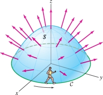
The laws of electricity and magnetism are expressed in terms of two vector fields, the electric field \({\bf{E}}\) and the magnetic field \({\bf{B}}\), whose properties are summarized in Maxwell’s four equations. One of these equations is Faraday’s Law of Induction, which can be formulated either as a partial differential equation or in the following “integral form”: \begin{equation*} \boxed{\int_{{\mathcal{C}}} {\bf{E}}\,{\cdot} d{\bf{s}} = -\frac{d }{d t}\iint_{{\mathcal{S}}\,} {\bf{B}}{\cdot} d{\bf{S}}}\tag{5} \end{equation*}
In this equation, \({\mathcal{S}}\) is an oriented surface with boundary curve \({\mathcal{C}}\), oriented as indicated in Figure 16.64. The line integral of \({\bf{E}}\) is equal to the voltage drop around the boundary curve (the work performed by \({\bf{E}}\) moving a positive unit charge around~\({\mathcal{C}}\)).
The tesla (T) is the SI unit of magnetic field strength. A one-coulomb point charge passing through a magnetic field of 1 T at 1 m/s experiences a force of 1 newton.
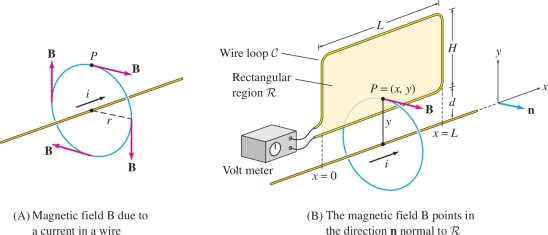
To illustrate Faraday’s Law, consider an electric current of \(i\) amperes flowing through a straight wire. According to the Biot-Savart Law, this current produces a magnetic field \({\bf{B}}\) of magnitude \(B(r)=\frac{\mu_0|i|}{2\pi r}\) T, where \(r\) is the distance (in meters) from the wire and \(\mu_0 = 4\pi\cdot 10^{-7}~\mathrm{\hbox{T-m}/A}\). At each point \(P\), \({\bf{B}}\) is tangent to the circle through \(P\) perpendicular to the wire as in Figure 16.65, with direction determined by the right-hand rule: If the thumb of your right hand points in the direction of the current, then your fingers curl in the direction of \({\bf{B}}\).
996
The electric field \({\bf{E}}\) is conservative when the charges are stationary or, more generally, when the magnetic field \({\bf{B}}\) is constant. When \({\bf{B}}\) varies in time, the integral on the right in Eq. (5) is nonzero for some surface, and hence the circulation of \({\bf{E}}\) around the boundary curve \({\mathcal{C}}\) is also nonzero. This shows that \({\bf{E}}\) is not conservative when \({\bf{B}}\) varies in time.
EXAMPLE 5
A varying current of magnitude (\(t\) in seconds) \[ i=28\cos\left(400t\right) \textrm{amperes} \] flows through a straight wire [Figure 16.65]. A rectangular wire loop \({\mathcal{C}}\) of length \(L=1.2~\mathrm{m}\) and width \(H=0.7~\mathrm{m}\) is located a distance \(d=0.1~\mathrm{m}\) from the wire as in the figure. The loop encloses a rectangular surface \({\mathcal{R}}\), which is oriented by normal vectors pointing out of the page.
- (a) Calculate the flux \(\Phi(t)\) of \({\bf{B}}\) through \({\mathcal{R}}\).
- (b) Use Faraday’s Law to determine the voltage drop (in volts) around the loop~\({\mathcal{C}}\).
Magnetic flux as a function of time is often denoted by the Greek letter \(\Phi\): \[ \Phi(t) = \iint_{{\mathcal{S}}\,} {\bf{B}}\cdot d{\bf{S}} \]
Solution We choose coordinates \((x,y)\) on rectangle \({\mathcal{R}}\) as in Figure 16.65, so that \(y\) is the distance from the wire and \({\mathcal{R}}\) is the region \[ 0\le x \le L,\qquad d \le y \le H + d \]
Our parametrization of \({\mathcal{R}}\) is simply \(G(x,y)=(x,y)\), for which the normal vector \({\bf{n}}\) is the unit vector perpendicular to \({\mathcal{R}}\), pointing out of the page. The magnetic field \({\bf{B}}\) at \(P=(x,y)\) has magnitude \(\frac{\mu_0|i|}{2\pi y}\). It points out of the page in the direction of \({\bf{n}}\) when \(i\) is positive and into the page when \(i\) is negative. Thus, \[ {\bf{B}} = \frac{\mu_0i}{2\pi y}{\bf{n}} \qquad\textrm{and}\qquad {\bf{B}}{\cdot}{\bf{n}} = \frac{\mu_0i}{2\pi y} \]
- (a) The flux \(\Phi(t)\) of \({\bf{B}}\) through \({\mathcal{R}}\) at time \(t\) is \[ \begin{array}{rl} \Phi(t) &= \iint_{{\mathcal{R}}\,} {\bf{B}}\cdot d{\bf{S}}= \int_{x=0}^L\int_{y=d}^{H+d} {\bf{B}}\cdot {\bf{n}}\,dy\,dx\\ &=\int_{x=0}^L\int_{y=d}^{H+d} \frac{\mu_0i}{2\pi y}\,dy\,dx = \frac{\mu_0Li}{2\pi}\int_{y=d}^{H+d} \frac{dy}{y} \\ &= \frac{\mu_0L}{2\pi}\left(\ln\frac{H+d}{d}\right) i \\ &= \frac{\mu_0(1.2)}{2\pi} \left(\ln\frac{0.8}{0.1}\right) 28 \cos\left(400t\right) \end{array} \] With \(\mu_0 = 4\pi\cdot 10^{-7}\), we obtain \[ \Phi(t) \approx 1.4 \times 10^{-5}\cos\left(400t\right)~\mathrm{T\hbox{-}m^2} \]
- (b) By Faraday’s Law [Eq. (5)], the voltage drop around the rectangular loop \({\mathcal{C}}\), oriented in the counterclockwise direction, is \[ \int_{{\mathcal{C}}} {\bf{E}}{\cdot}\,d{\bf{s}} = -\frac{d \Phi}{d t} \approx -(1.4 \times 10^{-5}) \left(400\right)\sin \left(400 t\right) = -0.0056\sin\left(400t\right)~\mathrm{V} \]
997
16.5.1 Summary
- A surface \({\mathcal{S}}\) is oriented if a continuously varying unit normal vector \({\bf{e}}_{{\bf{n}}}(P)\) is specified at each point on \({\mathcal{S}}\). This distinguishes an “outward” direction on the surface.
- The integral of a vector field \({\bf{F}}\) over an oriented surface \({\mathcal{S}}\) is defined as the integral of the normal component \({\bf{F}}{\cdot}{\bf{e}}_{{\bf{n}}}\) over \({\mathcal{S}}\).
- Vector surface integrals are computed using the formula \[ \iint_{{\mathcal{S}}\,}{\bf{F}}{\cdot} d{\bf{S}} = \iint_{{\mathcal{D}}\,} {\bf{F}}({G}(u,v)){\cdot} {\bf{n}}(u,v) \,du\,dv \] Here, \({G}(u,v)\) is a parametrization of \({\mathcal{S}}\) such that \({\bf{n}}(u,v)={\bf{T}}_u{\times}{\bf{T}}_v\) points in the direction of the unit normal vector specified by the orientation.
- The surface integral of a vector field \({\bf{F}}\) over \({\mathcal{S}}\) is also called the flux of \({\bf{F}}\) through \({G}\). If \({\bf{F}}\) is the velocity field of a fluid, then \(\iint_{{\mathcal{S}}\,}{\bf{F}}{\cdot} d{\bf{S}}\) is the rate at which fluid flows through \({\mathcal{S}}\) per unit time.