17.8 Divergence Theorem
We have studied several “Fundamental Theorems.” Each of these is a relation of the type: \[ \textrm{Integral of a derivative on an oriented domain} {\,}={\,} \textrm{Integral over the} {\it oriented} {\it boundary} \textrm{of the domain} \]
Here are the examples we have seen so far:
- In single-variable calculus, the Fundamental Theorem of Calculus (FTC) relates the integral of \(f'(x)\) over an interval \([a,b]\) to the “integral” of \(f(x)\) over the boundary of \([a,b]\) consisting of two points \(a\) and \(b\): \[ \underbrace{\int_a^b f'(x)\,dx}_{\textrm{Integral of derivative over \([a,b]\)}} = \underbrace{f(b)-f(a)}_{\textrm{“Integral” over the boundary of \([a,b]\)}} \] The boundary of \([a,b]\) is oriented by assigning a plus sign to \(b\) and a minus sign to \(a\).
- The Fundamental Theorem for Line Integrals generalizes the FTC: Instead of an interval \([a,b]\) (a path from \(a\) to
\(b\) along the \(x\)-axis), we take any path from points \(P\) to \(Q\) in \({\bf R}^3\) (Figure 17.53),
and instead of \(f'(x)\) we use the gradient:
\[
\underbrace{\int_{C} \nabla V
\cdot d{\bf s}}_{\textrm{Integral of derivative over a curve}}
= \underbrace{ V(Q)- V(P)}_
\textrm{“Integral” over the boundary \(\partial C = Q-P\)}
\]
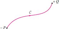 Figure 17.53: The oriented boundary of \(C\) is \(\partial C = Q-P\).
 - Green’s Theorem is a two-dimensional version of the FTC that relates the integral
of a derivative over a domain \(D\) in the plane to an integral over its boundary
curve \(C = \partial D\) (Figure 17.54):
\[ \underbrace{\iint_{D\,} \left(\dfrac{\partial{F_2}}{\partial{y}} - \dfrac{\partial{F_1}}{\partial{x}}\right) dA}_{\textrm{Integral of derivative over domain}} = \underbrace{\int_{C} {\bf F} \cdot d{\bf s}}_{\textrm{Integral over boundary curve}} \]
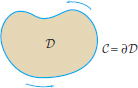 Figure 17.54: Domain \(D\) in \({\bf R}^2\) with boundary curve \(C=\partial D\).
 - Stokes’ Theorem extends Green’s Theorem: Instead of a domain in the plane (a flat surface), we allow
any surface in \({\bf R}^3\) (Figure 17.55). The appropriate derivative is the curl:
\[ \underbrace{\iint_{S\,} {\bf curl}({\bf F}) \cdot d{\bf S}}_{\textrm{Integral of derivative over surface}} = \underbrace{\int_{C} {\bf F} \cdot d{\bf s}}_{\textrm{Integral over boundary curve}} \]
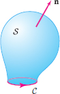 Figure 17.55: The oriented boundary of \(S\) is \(C=\partial S\).
Our last theorem—the Divergence Theorem—follows this pattern: \[ \underbrace{\iiint_{W\,} \hbox{div}({\bf F}) \, dW}_{\textrm{Integral of derivative over 3-D region}} = \underbrace{\iint_{S} {\bf F} \cdot d{\bf S}}_{\textrm{Integral over boundary surface}} \]
1029
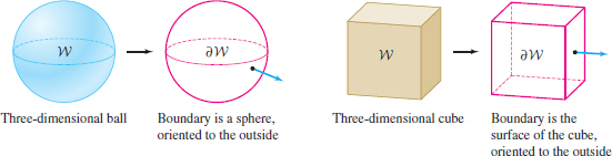
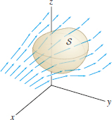
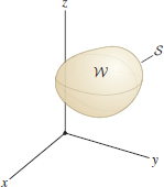
Here, \(S\) is a closed surface that encloses a \(3\)-D region \(W\). In other words, \(S\) is the boundary of \(W\): \(S = \partial W\). Recall that a closed surface is a surface that “holds air.” Figure 17.56 shows two examples of regions and boundary surfaces that we will consider.
The derivative appearing in the Divergence Theorem is the divergence of a vector field \({\bf F}=\langle F_1,F_2,F_3 \rangle\), defined by \begin{equation} \boxed{ \hbox{div}({\bf F})=\dfrac{\partial{F_1}}{\partial{x}}+\dfrac{\partial{F_2}}{\partial{y}}+ \dfrac{\partial{F_3}}{\partial{z}}}\tag{1} \end{equation}
Note
More advanced treatments of vector calculus use the theory of “differential forms” to formulate a general version of Stokes’ Theorem that is valid in all dimensions and includes each of our main theorems (Green’s, Stokes’, Divergence) as a special case.
We often write the divergence as a symbolic dot product: \[ \nabla\cdot{\bf F} = \langle \dfrac{\partial}{\partial{x}}, \dfrac{\partial}{\partial{y}}, \dfrac{\partial}{\partial{z}}\rangle \cdot \langle F_1, F_2, F_3 \rangle = \dfrac{\partial{F_1}}{\partial{x}}+\dfrac{\partial{F_2}}{\partial{y}}+ \dfrac{\partial{F_3}}{\partial{z}} \]
Note that, unlike the gradient and curl, the divergence is a scalar function. Like the gradient and curl, the divergence obeys the linearity rules: \begin{align*} \hbox{div}({\bf F}+{\bf G}) &= \hbox{div}({\bf F}) + \hbox{div}({\bf G})\\ \hbox{div}(c{\bf F}) &= c \, \hbox{div}({\bf F})\qquad \textrm{(\(c\) any constant)} \end{align*}
EXAMPLE 1
Evaluate the divergence of \({\bf F} = \langle e^{xy}, xy,z^4\rangle\) at \(P=(1,0,2)\).
Solution \begin{align*} \hbox{div}({\bf F}) &= \dfrac{\partial{}}{\partial{x}}\, e^{xy} + \dfrac{\partial}{\partial{y}}\, xy + \dfrac{\partial}{\partial{z}}\,z^4 = ye^{xy}+x+4z^3\\ \hbox{div}({\bf F})(P) &= \hbox{div}({\bf F})(1,0,2) = 0\cdot e^0+1+4\cdot 2^3 = 33 \end{align*}
THEOREM 1 Divergence Theorem
Let \(S\) be a closed surface that encloses a region \(W\) in \({\bf R}^3\). Assume that \(S\) is piecewise smooth and is oriented by normal vectors pointing to the outside of \(W\). Let \({\bf F}\) be a vector field whose domain contains \(W\). Then \begin{equation} \iint_{S\,} {\bf F} \cdot d{\bf S} = \iiint_{W\,} \hbox{div}({\bf F})\, dV\tag{2} \end{equation}
Proof
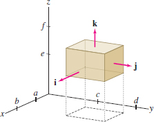
We prove the Divergence Theorem in the special case that \(W\) is a box \([a,b]\times[c,d]\times[e,f]\) as in Figure 17.57. The proof can be modified to treat more general regions such as the interiors of spheres and cylinders.
1030
We write each side of Eq. (2) as a sum over components: \begin{eqnarray*} \iint_{\partial W}(F_1{\bf i}+F_2{\bf j}+F_3{\bf k})\cdot d{\bf S} &=& \iint_{\partial W}\! F_1{\bf i}\cdot d{\bf S} + \iint_{\partial W}\! F_2{\bf j}\cdot d{\bf S} + \iint_{\partial W}\! F_3{\bf k}\cdot d{\bf S} \\ \iiint_{W} \hbox{div}(F_1{\bf i}+F_2{\bf j}+F_3{\bf k})\, dV &=& \iiint_{W} \hbox{div}(F_1{\bf i})\, dV + \iiint_{W} \hbox{div}(F_2{\bf j})\, dV \\ &&{} + \iiint_{W} \hbox{div}(F_3{\bf k})\, dV \end{eqnarray*}
REMINDER
The Divergence Theorem states \[\iint_{S\,} {\bf F} \cdot d{\bf S} = \iiint_{W\,} \hbox{div}({\bf F})\, dV\]
As in the proofs of Green’s and Stokes’ Theorems, we show that corresponding terms are equal. It will suffice to carry out the argument for the \({\bf i}\)-component (the other two components are similar). Thus we assume that \({\bf F} = F_1{\bf i}\).
The surface integral over boundary \(S\) of the box is the sum of the integrals over the six faces. However, \({\bf F}=F_1{\bf i}\) is orthogonal to the normal vectors to the top and bottom as well as the two side faces because \(\displaystyle{ {\bf F}\cdot{\bf j} ={\bf F}\cdot{\bf k} = 0}\). Therefore, the surface integrals over these faces are zero. Nonzero contributions come only from the front and back faces, which we denote \(S_f\) and \(S_b\) (Figure 17.58): \[ \iint_{S\,} {\bf F}\cdot d{\bf S} = \iint_{S_f\,} {\bf F}\cdot d{\bf S} + \iint_{S_b\,} {\bf F}\cdot d{\bf S} \]
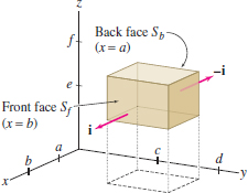
To evaluate these integrals, we parametrize \(S_f\) and \(S_b\) by \begin{align*} G_f(y,z) &=(b,y,z),&\qquad& c \le y \le d,\ e \le z \le f\\ G_b(y,z) &=(a,y,z),&\qquad&c \le y \le d,\ e \le z \le f \end{align*}
The normal vectors for these parametrizations are \begin{align*} \dfrac{\partial{G_f}}{\partial{y}}\times\dfrac{\partial{G_f}}{\partial{z}} &= {\bf j}\times{\bf k} = {\bf i}\\ \dfrac{\partial{G_b}}{\partial{y}}\times\dfrac{\partial{G_b}}{\partial{z}} &= {\bf j}\times{\bf k} = {\bf i} \end{align*}
However, the outward-pointing normal for \(S_b\) is \(-{\bf i}\), so a minus sign is needed in the surface integral over \(S_b\) using the parametrization \(G_b\): \begin{align*} \iint_{S_f\,} {\bf F}\cdot d{\bf S} +\iint_{S_b\,} {\bf F}\cdot d{\bf S} &= \int_e^f\int_c^d F_1(b,y,z)\,dy\,dz -\int_e^f\int_c^d F_1(a,y,z) \,dy\,dz\\ &= \int_e^f\int_c^d \Big(F_1(b,y,z)-F_1(a,y,z)\Big)\,dy\,dz \end{align*}
Note
The names attached to mathematical theorems often conceal a more complex historical development. What we call Green’s Theorem was stated by Augustin Cauchy in 1846 but it was never stated by George Green himself (he published a result that implies Green’s Theorem in 1828). Stokes’ Theorem first appeared as a problem on a competitive exam written by George Stokes at Cambridge University, but William Thomson (Lord Kelvin) had previously stated the theorem in a letter to Stokes. Gauss published special cases of the Divergence Theorem in 1813 and later in 1833 and 1839, while the general theorem was stated and proved by the Russian mathematician Michael Ostrogradsky in 1826. For this reason, the Divergence Theorem is also referred to as “Gauss’s Theorem” or the “Gauss-Ostrogradsky Theorem.”
By the FTC in one variable, \[ F_1(b,y,z)-F_1(a,y,z) = \int_a^b\,\dfrac{\partial{F_1}}{\partial{x}}(x,y,z)\,dx \]
Since \(\displaystyle{\hbox{div}({\bf F})=\hbox{div}(F_1{\bf i})=\dfrac{\partial{F_1}}{\partial{x}}}\), we obtain the desired result: \begin{align*} \iint_{S\,} {\bf F}\cdot d{\bf S} = \int_e^f\int_c^d\int_a^b \dfrac{\partial{F_1}}{\partial{x}}(x,y,z) \,dx\,dy\,dz = \iiint_{W\,} \hbox{div}({\bf F})\,dV \end{align*}
1031
EXAMPLE 2 Verifying the Divergence Theorem
Verify Theorem 1 for \({\bf F} = \langle y,yz,z^2 \rangle\) and the cylinder in Figure 17.59.
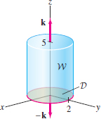
Solution We must verify that the flux \(\displaystyle{\iint_{S\,} {\bf F} \cdot d{\bf S}}\), where \(S\) is the boundary of the cylinder, is equal to the integral of \(\hbox{div}(W)\) over the cylinder. We compute the flux through \(S\) first: It is the sum of three surface integrals over the side, the top, and the bottom.
Step 1. Integrate over the side of the cylinder
We use the standard parametrization of the cylinder: \begin{align*} G(\theta,z) &=(2\cos\theta,2\sin\theta,z),\qquad 0\le\theta>2\pi,\quad 0 \le z\le 5 \end{align*}
The normal vector is \begin{align*} {\bf n} &= {\bf T}_{\theta} \times {\bf T}_z = \langle -2\sin\theta,2\cos\theta,0 \rangle \times \langle 0,0,1 \rangle = \langle 2\cos\theta,2\sin\theta,0 \rangle \end{align*} and \({\bf F}(G(\theta,z)) = \langle y,yz,z^2 \rangle =\langle 2\sin\theta,2z\sin\theta,z^2 \rangle\). Thus \begin{align} {\bf F} \cdot d{\bf S}& = \langle 2\sin\theta,2z\sin\theta,z^2 \rangle \cdot \langle 2\cos\theta,2\sin\theta,0 \rangle\,d\theta\,dz\notag \\[4pt] &= 4\cos\theta\sin\theta + 4z\sin^2\theta\,d\theta\,dz\notag \\[4pt] \iint_{\textrm{side}} {\bf F} \cdot d{\bf S} &= \int_0^5\int_0^{2\pi} (4\cos\theta\sin\theta + 4z\sin^2\theta)\,d\theta\,dz\notag \\[4pt] &= 0 + 4\pi\int_0^5 z \,dz = 4\pi\left(\frac{25}2\right) = 50\pi\tag{3} \end{align}
Step 2. Integrate over the top and bottom of the cylinder
The top of the cylinder is at height \(z=5\), so we can parametrize the top by \(G(x,y)=(x, y,5)\) for \((x,y)\) in the disk \(D\) of radius \(2\): \[ D = \{(x,y):x^2+y^2\le 4\} \]
REMINDER
In Eq. (3), we use \begin{align*} \int_0^{2\pi} \cos\theta\sin\theta\,d\theta & = 0 \\ \int_0^{2\pi} \sin^2\theta\,d\theta &=\pi \end{align*}
Then \begin{align*} {\bf n} &= {\bf T}_x \times {\bf T}_y = \langle 1,0,0 \rangle \times \langle 0,1,0 \rangle = \langle 0,0,1 \rangle \end{align*} and since \({\bf F}(G(x,y)) ={\bf F}(x,y,5) = \langle y,5y,5^2 \rangle\), we have \begin{align*} {\bf F}(G(x,y)) \cdot {\bf n} &= \langle y,5y,5^2 \rangle \cdot \langle 0,0,1 \rangle = 25\\ \iint_{\textrm{top}} {\bf F}\cdot d{\bf S} &= \iint_{D\,} 25\,dA = 25\,\mathrm{Area}(D) = 25(4\pi)=100\pi \end{align*}
Along the bottom disk of the cylinder, we have \(z=0\) and \({\bf F}(x, y, 0) = \langle y, 0 , 0\rangle\). Thus \({\bf F}\) is orthogonal to the vector \(-{\bf k}\) normal to the bottom disk, and the integral along the bottom is zero.
Step 3. Find the total flux \[ \iint_{S\,} {\bf F} \cdot d{\bf S} = \textrm{sides \(+\) top \(+\) bottom} = 50\pi+100\pi +0=\boxed{150\pi} \]
Step 4. Compare with the integral of divergence \[ \hbox{div}({\bf F}) = \hbox{div}\bigl(\langle y, yz, z^2\rangle\bigr)=\dfrac{\partial}{\partial{x}}y+\dfrac{\partial}{\partial{y}}(yz)+\dfrac{\partial}{\partial{z}}z^2 = 0+z+2z=3z \]
1032
The cylinder \(W\) consists of all points \((x,y,z)\) for \(0\le z\le 5\) and \((x,y)\) in the disk \(D\). We see that the integral of the divergence is equal to the total flux as required: \begin{align*} \iiint_{W\,}\hbox{div}({\bf F})\,dV &= \iint_{D\,}\int_{z=0}^5 3z\,dV = \iint_{D\,} \frac{75}2\,dA \\ &= \left(\frac{75}2\right)(\textrm{Area}(D)) = \left(\frac{75}2\right)(4\pi) = \boxed{150\pi} \end{align*}
In many applications, the Divergence Theorem is used to compute flux. In the next example, we reduce a flux computation (that would involve integrating over six sides of a box) to a more simple triple integral.
EXAMPLE 3 Using the Divergence Theorem
Use the Divergence Theorem to evaluate \(\displaystyle{\iint_{S\,} \langle x^2,z^4,e^z\rangle\cdot d{\bf S}}\), where \(S\) is the boundary of the box \(W\) in Figure 17.60.
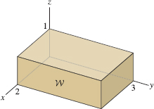
Solution First, compute the divergence: \[ \hbox{div}\bigl(\langle x^2,z^4,e^z\rangle\bigr) = \dfrac{\partial}{\partial{x}}\,x^2 + \dfrac{\partial}{\partial{y}}\,z^4 + \dfrac{\partial}{\partial{z}}\,e^z = 2x+e^z \]
Then apply the Divergence Theorem and use Fubini’s Theorem: \begin{align*} \iint_{S\,} \langle x^2,z^4,e^z\rangle\cdot d{\bf S} &= \iiint_{W\,} (2x+e^z)\,dV= \int_0^2\int_0^3\int_0^1(2x+e^z)\,dz\,dy\,dx\\ &= 3\int_0^2 2x \,dx + 6\int_0^1 e^z\,dz = 12+6(e-1)=6e+6 \end{align*}
EXAMPLE 4 A Vector Field with Zero Divergence
Compute the flux of \[ {\bf F} = \langle z^2+xy^2, \cos(x+z), e^{-y}-zy^2\rangle \] through the boundary of the surface \(S\) in Figure 17.61.
Solution Although \({\bf F}\) is rather complicated, its divergence is zero: \[ \hbox{div}({\bf F}) = \dfrac{\partial{}}{\partial{x}}(z^2+xy^2)+ \dfrac{\partial{}}{\partial{y}}\cos(x+z)+\dfrac{\partial{}}{\partial{z}}(e^{-y}-zy^2) = y^2-y^2 = 0 \]
The Divergence Theorem shows that the flux is zero. Letting \(W\) be the region enclosed by \(S\), we have \[ \iint_{S\,} {\bf F} \cdot d{\bf S} = \iiint_{W\,} \hbox{div}({\bf F})\, dV = \iiint_{W\,} 0\, dV = 0 \]
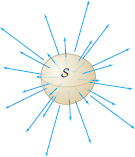
GRAPHICAL INSIGHT Interpretation of Divergence
Let’s assume again that \({\bf F}\) is the velocity field of a fluid (Figure 17.62). Then the flux of \({\bf F}\) through a surface \(S\) is the flow rate (volume of fluid passing through \(S\) per unit time). If \(S\) encloses the region \(W\), then by the Divergence Theorem, \begin{equation} \textrm{Flow rate across \(S\)} = \iiint_{W\,}\hbox{div}({\bf F})\,dV\tag{4} \end{equation}
Now assume that \(S\) is a small surface containing a point \(P\). Because \(\displaystyle{\hbox{div}({\bf F})}\) is continuous (it is a sum of derivatives of the components of \({\bf F}\)), its value does not change much on \(W\) if \(S\) is sufficiently small and to a first approximation, we can replace \(\hbox{div}({\bf F})\) by the constant value \(\hbox{div}({\bf F})(P)\). This gives us the approximation \begin{equation} \textrm{Flow rate across \(S\)} = \iiint_{W\,}\hbox{div}({\bf F})\,dV \approx \hbox{div}({\bf F})(P)\,\cdot\,\textrm{Vol}(W)\tag{5} \end{equation}
1033
In other words, the flow rate through a small closed surface containing \(P\) is approximately equal to the divergence at \(P\) times the enclosed volume, and thus \(\hbox{div}({\bf F})(P)\) has an interpretation as “flow rate (or flux) per unit volume”:
- If \(\hbox{div}({\bf F})(P)>0\), there is a net outflow of fluid across any small closed surface enclosing \(P\), or, in other words, a net “creation” of fluid near \(P\).
- If \(\hbox{div}({\bf F})(P)<0\), there is a net inflow of fluid across any small closed surface enclosing \(P\), or, in other words, a net “destruction” of fluid near \(P\).
Because of this, \(\hbox{div}({\bf F})\) is sometimes called the source density of the field.
- If \(\hbox{div}({\bf F})(P)=0\), then to a first-order approximation, the net flow across any small closed surface enclosing \(P\) is equal to zero.
A vector field such that \(\hbox{div}({\bf F}) = 0\) everywhere is called incompressible.
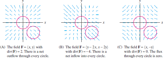
To visualize these cases, consider the two-dimensional situation, where we define \[\displaystyle \hbox{div}(\langle F_1, F_2\rangle)=\dfrac{\partial{F_1}}{\partial{x}}+\dfrac{\partial{F_2}}{\partial{y}}\]
In Figure 17.63, field (A) has positive divergence. There is a positive net flow of fluid across every circle per unit time. Similarly, field (B) has negative divergence. By contrast, field (C) is incompressible. The fluid flowing into every circle is balanced by the fluid flowing out.
Note
Do the units match up in Eq. (5)? The flow rate has units of volume per unit time. On the other hand, the divergence is a sum of derivatives of velocity with respect to distance. Therefore, the divergence has units of “distance per unit time per distance,” or unit time\(^{-1}\), and the right-hand side of Eq. (5) also has units of volume per unit time.
Applications to Electrostatics
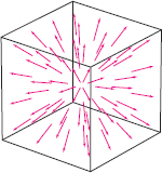
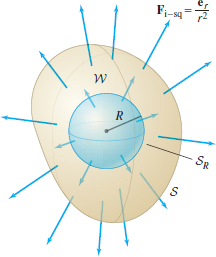
The Divergence Theorem is a powerful tool for computing the flux of electrostatic fields. This is due to the special properties of the inverse-square vector field (Figure 17.64). In this section, we denote the inverse-square vector field by \(\displaystyle{{\bf F}_{\textrm{i-sq}}}\): \[\boxed{ {\bf F}_{\textrm{i-sq}}=\frac{{\bf e}_r}{r^2} }\] Recall that \({\bf F}_{\textrm{i-sq}}\) is defined for \(r\ne 0\). The next example verifies the key property that \(\hbox{div}({\bf F}_{\textrm{i-sq}})=0\).
REMINDER
\[ r=\sqrt{x^2+y^2+z^2} \] For \(r\ne 0\), \[ {\bf e}_r = \frac{\langle x, y, z\rangle}{r} = \frac{\langle x, y, z\rangle}{\sqrt{x^2+y^2+z^2}} \]
1034
EXAMPLE 5 The Inverse-Square Vector Field
Verify that \(\displaystyle{{\bf F}_{\textrm{i-sq}}=\frac{{\bf e}_r}{r^2}}\) has zero divergence: \[ \hbox{div}\left(\frac{{\bf e}_r}{r^2}\right) = 0 \]
Solution Write the field as \[ {\bf F}_{\textrm{i-sq}} = \langle F_1, F_2, F_3\rangle = \frac1{r^2}\langle \frac{x}r,\frac{y}r, \frac{z}r\rangle = \langle xr^{-3},yr^{-3}, zr^{-3}\rangle \]
We have \begin{align*} \dfrac{\partial{r}}{\partial{x}} &= \dfrac{\partial}{\partial{x}}(x^2+y^2+z^2)^{1/2} = \frac12(x^2+y^2+z^2)^{-1/2}(2x)=\frac{x}r \\ \dfrac{\partial{F_1}}{\partial{x}} &= \dfrac{\partial}{\partial{x}} xr^{-3} = r^{-3} - 3xr^{-4}\dfrac{\partial{r}}{\partial{x}} = r^{-3} -(3xr^{-4})\frac{x}r = \frac{r^2-3x^2}{r^{5}} \end{align*}
The derivatives \(\displaystyle{\dfrac{\partial{F_2}}{\partial{y}}}\) and \(\displaystyle{\dfrac{\partial{F_3}}{\partial{z}}}\) are similar, so \[ \hbox{div}({\bf F}_{\textrm{i-sq}}) = \frac{r^2-3x^2}{r^{5}}+\frac{r^2-3y^2}{r^{5}}+\frac{r^2-3z^2}{r^{5}} = \frac{3r^2-3(x^2+y^2+z^2)}{r^{5}} = 0 \]
The next theorem shows that the flux of \({\bf F}_{\textrm{i-sq}}\) through a closed surface \(S\) depends only on whether \(S\) contains the origin.
THEOREM 2 Flux of the Inverse-Square Field
The flux of \(\displaystyle{{\bf F}_{\textrm{i-sq}}=\frac{{\bf e}_r}{r^2}}\) through closed surfaces has the following remarkable description: \[\boxed{ \iint_{S}\left(\frac{{\bf e}_r}{r^2}\right)\cdot\,d\,{\bf S} = \begin{cases} 4\pi \quad & \textrm{if \(S\) encloses the origin}\\ 0& \textrm{if \(S\) does not enclose the origin} \end{cases} }\]
Proof
First, assume that \(S\) does not contain the origin (Figure 17.65). Then the region \(W\) enclosed by \(S\) is contained in the domain of \({\bf F}_{\textrm{i-sq}}\) and we can apply the Divergence Theorem. By Example 5, \(\hbox{div}({\bf F}_{\textrm{i-sq}})=0\) and therefore \[ \iint_{S}\left(\frac{{\bf e}_r}{r^2}\right)\cdot\,d\,{\bf S} = \iiint_{W}\hbox{div}({\bf F}_{\textrm{i-sq}})\,dV = \iiint_{W}0\,\,dV =0 \]
Next, let \(S_R\) be the sphere of radius \(R\) centered at the origin (Figure 17.66). We cannot use the Divergence Theorem because \(S_R\) contains a point (the origin) where \({\bf F}_{\textrm{i-sq}}\) is not defined. However, we can compute the flux of \({\bf F}_{\textrm{i-sq}}\) through \(S_R\) using spherical coordinates. Recall from Section 16.4 [Eq. (5)] that the outward-pointing normal vector in spherical coordinates is \[ {\bf n} = {\bf T}_\phi\times {\bf T}_\theta = (R^2\sin\phi) {\bf e}_r \]

The inverse-square field on \(S_R\) is simply \({\bf F}_{\textrm{i-sq}} = R^{-2}{\bf e}_r\), and thus \[{\bf F}_{\textrm{i-sq}}\cdot {\bf n} = (R^{-2}{\bf e}_r)\cdot (R^2\sin\phi{\bf e}_r) = \sin\phi({\bf e}_r\cdot{\bf e}_r)=\sin\phi\] \begin{align*} \iint_{S_R\,}{\bf F}_{\textrm{i-sq}}\cdot d{\bf S} &= \int_0^{2\pi}\int_0^{\pi}{\bf F}_{\textrm{i-sq}}\cdot{\bf n}\,d\phi\,d\theta\\ &= \int_0^{2\pi}\int_{0}^{\pi}\sin\phi\,d\phi\,d\theta\\ & = 2\pi\int_{0}^{\pi}\sin\phi\,d\phi = 4\pi \end{align*}
1035
To extend this result to any surface \(S\) containing the origin, choose a sphere \(S_R\) whose radius \(R>0\) is so small that \(S_R\) is contained inside \(S\). Let \(W\) be the region between \(S_R\) and \(S\) (Figure 17.67). The oriented boundary of \(W\) is the difference \[ \partial W = S-S_R \]
This means that \(S\) is oriented by outward-pointing normals and \(S_R\) by inward-pointing normals. By the Divergence Theorem, \begin{align*} \iint_{\partial W}\,{\bf F}_{\textrm{i-sq}}\cdot\,d{\bf S} &=& \iint_{S\,}{\bf F}_{\textrm{i-sq}}\cdot d{\bf S} - \iint_{S_R\,}{\bf F}_{\textrm{i-sq}}\cdot d{\bf S}&\\ &= & \iiint_{W\,}\hbox{div}({\bf F}_{\textrm{i-sq}})\,dV\qquad&\textrm{(Divergence Theorem)} \\ &=& \iiint_{W\,} 0 \,dV = 0\qquad&\textrm{(Because \(\hbox{div}({\bf F}_{\textrm{i-sq}})=0\))} \end{align*}
Note
To verify that the Divergence Theorem remains valid for regions between two surfaces, such as the region \(W\) in Figure 17.67, we cut \(W\) down the middle. Each half is a region enclosed by a surface, so the the Divergence Theorem as we have stated it applies. By adding the results for the two halves, we obtain the Divergence Theorem for \(W\). This uses the fact that the fluxes through the common face of the two halves cancel.
This proves that the fluxes through \(S\) and \(S_R\) are equal, and hence both equal \(4\pi\).
Notice that we just applied the Divergence Theorem to a region \(W\) that lies between two surfaces, one contained in the other. This is a more general form of the theorem than the one we stated formally in Theorem 1 above. The marginal comment explains why this is justified.
This result applies directly to the electric field \({\bf E}\) of a point charge, which is a multiple of the inverse-square vector field. For a charge of \(q\) coulombs at the origin, \[ {\bf E} = \left(\frac{q}{4\pi\epsilon_0}\right) \frac{{\bf e}_r}{r^2} \] where \(\epsilon_0=8.85\times 10^{-12} \text{C\(^2\)/N-m}^2\) is the permittivity constant. Therefore, \[ \textrm{Flux of \({\bf E}\) through \(S\)} = \begin{cases} \dfrac{q}{\epsilon_0} & \textrm{if \(q\) is inside \(S\)}\\ 0 \quad & \textrm{if \(q\) is outside \(S\)} \end{cases} \]
Now, instead of placing just one point charge at the origin, we may distribute a finite number \(N\) of point charges \(q_i\) at different points in space. The resulting electric field \({\bf E}\) is the sum of the fields \({\bf E}_i\) due to the individual charges, and \[ \iint_{S\,}{\bf E}\cdot d{\bf S} = \iint_{S\,}{\bf E}_1\cdot d{\bf S}+\cdots+ \iint_{S\,}{\bf E}_N\cdot d{\bf S} \]
Each integral on the right is either \(0\) or \(\displaystyle{{q_i}/{\epsilon_0}}\), according to whether or not \(S\) contains \(q_i\), so we conclude that \begin{equation} \boxed{ \iint_{S\,}{\bf E}\cdot d{\bf S} = \frac{\textrm{total charge enclosed by \(S\)}}{\epsilon_0}}\tag{6} \end{equation}
This fundamental relation is called Gauss’s Law. A limiting argument shows that Eq. (6) remains valid for the electric field due to a continuous distribution of charge.
The next theorem, describing the electric field due to a uniformly charged sphere, is a classic application of Gauss’s Law.
1036
THEOREM 3 Uniformly Charged Sphere
The electric field due to a uniformly charged hollow sphere \(S_R\) of radius \(R\), centered at the origin and of total charge \(Q\), is \begin{equation} {\bf E} = \begin{cases} \dfrac{Q}{4\pi\epsilon_0 r^2}{\bf e}_r& \textrm{if \(r >R\)}\\ \mathbf{0} & \textrm{if \(r < R\)}\tag{7} \end{cases} \end{equation} where \(\displaystyle{\epsilon_0=8.85\times 10^{-12} \mathrm{C^2\text{/}N\hbox{-}m}^2}\).
Proof
By symmetry (Figure 17.68), the electric field \({\bf E}\) must be directed in the radial direction \({\bf e}_r\) with magnitude depending only on the distance \(r\) to the origin. Thus, \({\bf E}=E(r){\bf e}_r\) for some function \(E(r)\). The flux of \({\bf E}\) through the sphere \(S_r\) of radius \(r\) is \[ \iint_{S_r\,} {\bf E} \cdot d{\bf S} = E(r)\underbrace{\iint_{S_r\,}{\bf e}_r\cdot d{\bf S}}_{\textrm{Surface area of sphere}} = 4\pi r^2 E(r) \]
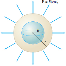
By Gauss’s Law, this flux is equal to \(C/\epsilon_0\), where \(C\) is the charge enclosed by \(S_r\). If \(r<R\), then \(C=0\) and \({\bf E}=\mathbf{0}\). If \(r>R\), then \(C=Q\) and \(4\pi r^2 E(r)=Q/\epsilon_0\), or \(\displaystyle{E(r)=Q/(\epsilon_04\pi r^2)}\). This proves Eq. (7).
Note
We proved Theorem 3 in the analogous case of a gravitational field (also a radial inverse-square field) by a laborious calculation in Exercise 48 of Section 16.4. Here, we have derived it from Gauss’s Law and a simple appeal to symmetry.
CONCEPTUAL INSIGHT
Here is a summary of the basic operations on functions and vector fields: \[ \boxed{ \begin{array} \(f & \overset{\nabla}{\longrightarrow} & {\bf F} & \overset{\textrm{curl}}{\longrightarrow} & {\bf G} & \overset{\textrm{div}}{\longrightarrow} & g\\ \hbox{function}&&\hbox{vector field}&&\hbox{vector field}&&\hbox{function} \end{array}}\]
One basic fact is that the result of two consecutive operations in this diagram is zero: \[ \boxed{ {\bf curl}(\nabla(f)) = {\bf 0},\qquad\hbox{div}({\bf curl}({\bf F})) = 0} \]
We verified the first identity in Example 1 of Section 17.2. The second identity is left as an exercise (Exercise 6).
An interesting question is whether every vector field satisfying \({\bf curl}({\bf F})={\bf 0}\) is necessarily conservative—that is, \({\bf F}=\nabla V\) for some function \( V\). The answer is yes, but only if the domain \(D\) is simply connected (every path can be drawn down to a point in \(D\)). We saw in Section 16.3 that the vortex vector satisfies \({\bf curl}({\bf F})={\bf 0}\) and yet cannot be conservative because its circulation around the unit circle is nonzero (the circulation of a conservative vector field is always zero). However, the domain of the vortex vector field is \({\bf R}^2\) with the origin removed, and this domain is not simply-connected.
The situation for vector potentials is similar. Can every vector field \({\bf G}\) satisfying \(\hbox{div}({\bf G}) = \textbf{0}\) be written in the form \({\bf G} = {\bf curl}({\bf A})\) for some vector potential \({\bf A}\)? Again, the answer is yes—provided that the domain is a region \(W\) in \({\bf R}^3\) that has “no holes,” like a ball, cube, or all of \({\bf R}^3\). The inverse-square field \({\bf F}_{\textrm{i-sq}} = {\bf e}_r/r^2\) plays the role of vortex field in this setting: Although \(\hbox{div}({\bf F}_{\textrm{i-sq}})=0\), \({\bf F}_{\textrm{i-sq}}\) cannot have a vector potential because its flux through the unit sphere is nonzero as shown in Theorem 2 (the flux over a closed surface of a vector field with a vector potential is always zero by Theorem 2 of Section 17.2). In this case, the domain of \({\bf e}_r/r^2\) is \({\bf R}^3\) with the origin removed, which “has a hole.”
These properties of the vortex and inverse-square vector fields are significant because they relate line and surface integrals to “topological” properties of the domain, such as whether the domain is simply-connected or has holes. They are a first hint of the important and fascinating connections between vector analysis and the area of mathematics called topology.
1037
HISTORICAL PERSPECTIVE
Vector analysis was developed in the nineteenth century, in large part, to express the laws of electricity and magnetism. Electromagnetism was studied intensively in the period 1750–1890, culminating in the famous Maxwell Equations, which provide a unified understanding in terms of two vector fields: the electric field \({\bf E}\) and the magnetic field \({\bf B}\). In a region of empty space (where there are no charged particles), the Maxwell Equations are \[ \boxed{ \begin{array} \!\!\hbox{div}({\bf E})&{}={}&0,& \hbox{div}({\bf B})&{}={}&0\\ \!\!{\bf curl}({\bf E}) &=& -\dfrac{\partial{\bf B}}{\partial{t}},& {\bf curl}({\bf B}) &=& \mu_0\epsilon_0\dfrac{\partial{\bf E}}{\partial{t}}\!\! \end{array}} \] where \(\mu_0\) and \(\epsilon_0\) are experimentally determined constants. In SI units, \begin{align*} \mu_0 &= 4\pi\times 10^{-7} \text{henries/m}\\ \epsilon_0 &\approx 8.85 \times 10^{-12} \text{farads/m} \end{align*}
Note
This is not just mathematical elegance\(\dots\) but beauty. It is so simple and yet it describes something so complex.
Francis Collins (1950– ), leading geneticist and former director of the Human Genome Project, speaking of the Maxwell Equations.
These equations led Maxwell to make two predictions of fundamental importance: (1) that electromagnetic waves exist (this was confirmed by H. Hertz in 1887), and (2) that light is an electromagnetic wave.
How do the Maxwell Equations suggest that electromagnetic waves exist? And why did Maxwell conclude that light is an electromagnetic wave? It was known to mathematicians in the eighteenth century that waves traveling with velocity \(c\) may be described by functions \(\varphi(x,y,z,t)\) that satisfy the wave equation \[ \boxed{ \Delta\varphi = \frac{1}{c^2}\dfrac{\partial{^2\varphi}}{\partial{t^2}}}\tag{8} \] where \(\Delta\) is the Laplace operator (or “Laplacian”) \[{\Delta\varphi = \dfrac{\partial{^2\varphi}}{\partial{x^2}}+\dfrac{\partial{^2\varphi}}{\partial{y^2}}+\dfrac{\partial{^2\varphi}}{\partial{z^2}}}\]
We will show that the components of \({\bf E}\) satisfy this wave equation. Take the curl of both sides of Maxwell’s third equation: \[ {\bf curl}({\bf curl}({\bf E})) = {\bf curl}\left(-\dfrac{\partial{\bf B}}{\partial{t}}\right) = -\dfrac{\partial{}}{\partial{t}} {\bf curl}({\bf B}) \]
Then apply Maxwell’s fourth equation to obtain \begin{eqnarray} {\bf curl}({\bf curl}({\bf E})) &=& -\dfrac{\partial{}}{\partial{t}}\left(\mu_0\epsilon_0\dfrac{\partial{\bf E}}{\partial{t}}\right)\notag\\ &=& -\mu_0\epsilon_0\dfrac{\partial{^2{\bf E}}}{\partial{t^2}}\tag{9} \end{eqnarray}
Finally, let us define the Laplacian of a vector field \[ {\bf F}=\langle F_1,F_2,F_3 \rangle \] by applying the Laplacian \(\Delta\) to each component, \(\displaystyle{\Delta{\bf F}=\langle \Delta F_1,\Delta F_2,\Delta F_3 \rangle}\). Then the following identity holds (see Exercise 36): \[ {\bf curl}({\bf curl}({\bf F}))=\nabla(\hbox{div}({\bf F}))-\Delta{\bf F} \]
Applying this identity to \({\bf E}\), we obtain \({\bf curl}({\bf curl}({\bf E}))=-\Delta{\bf E}\) because \(\hbox{div}({\bf E})=0\) by Maxwell’s first equation. Thus, Eq. (9) yields \[\boxed{ \Delta {\bf E} = \mu_0\epsilon_0\dfrac{\partial{^2{\bf E}}}{\partial{t^2}} }\]
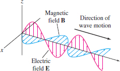
In other words, each component of the electric field satisfies the wave equation (8), with \(c=(\mu_0\epsilon_0)^{-1/2}\). This tells us that the \({\bf E}\)-field (and similarly the \({\bf B}\)-field) can propagate through space like a wave, giving rise to electromagnetic radiation (Figure 17.69).
Maxwell computed the velocity \(c\) of an electromagnetic wave: \[ c=(\mu_0\epsilon_0)^{-1/2}\approx 3\times 10^8 \text{m/s} \] and observed that the value is suspiciously close to the velocity of light (first measured by Olaf Römer in 1676). This had to be more than a coincidence, as Maxwell wrote in 1862: “We can scarcely avoid the conclusion that light consists in the transverse undulations of the same medium which is the cause of electric and magnetic phenomena.” Needless to say, the wireless technologies that drive our modern society rely on the unseen electromagnetic radiation whose existence Maxwell first predicted on mathematical grounds.
1038