7.7 Probability and Integration
What is the probability that a customer will arrive at a fast-food restaurant in the next \(45\) seconds? Or of scoring above \(90\%\) on a standardized test? Probabilities such as these are described as areas under the graph of a function \(p(x)\) called a probability density function (Figure 7.17). The methods of integration developed in this chapter are used extensively in the study of such functions.
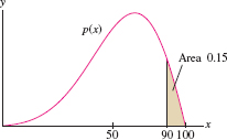
In probability theory, the quantity \(X\) that we are trying to predict (time to arrival, exam score, etc.) is called a random variable. The probability that \(X\) lies in a given range \([a,b]\) is denoted \[ P~(a\le X \le b) \]
For example, the probability of a customer arriving within the next \(30\) to \(45\) seconds is denoted \(P~(30 \le X \le 45)\).
We say that \(X\) is a continuous random variable if there is a continuous probability density function \(p(x)\) such that \[ P(a\le X \le b) = \int_a^b\,p(x)\,dx \]
A probability density function \(p(x)\) must satisfy two conditions. First, it must satisfy \(p(x)\ge 0\) for all \(x\), because a probability cannot be negative. Second, \[ \boxed{\bbox[#FAF8ED,5pt]{\int_{-\infty}^{\infty}p(x) = 1}}\tag{1} \]
The integral represents \(P(-\infty<X<\infty)\). It must equal 1 because it is certain (the probability is \(1\)) that the value of \(X\) lies between \(-\infty\) and \(\infty\).
We write \(P(X\le b)\) for the probability that \(X\) is at most \(b\), and \(P(X\ge b)\) for the probability that \(X\) is at least \(b\).
EXAMPLE 1
Find a constant \(C\) for which \(p(x) = \frac{C}{x^2+1}\) is a probability density function. Then compute \(P(1\le X\le 4)\).
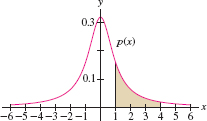
Solution We must choose \(C\) so that Eq. (1) is satisfied. The improper integral is a sum of two integrals (see marginal note) \[ \int_{-\infty}^{\infty} p(x)\,dx = C\int_{-\infty}^{0} \frac{\,dx}{x^2+1} + C\int_{0}^{\infty} \frac{\,dx}{x^2+1} = C\frac{\pi}2 + C\frac{\pi}2 = C\pi \]
Therefore, Eq. (1) is satisfied if \(C\pi =1\) or \(C=\pi^{-1}\). We have \[ P(1<X<4) = \int_1^4 p(x)\,dx = \int_1^4 \frac{\pi^{-1}\,dx}{x^2+1} = \pi^{-1}(\tan^{-1}4-\tan^{-1}1) \approx 0.17 \]
Therefore, \(X\) lies between \(1\) and \(4\) with probability \(0.17\), or \(17\%\) (Figure 7.18).
Reminder
\[ \begin{align*} \int_{-\infty}^{0}\frac{\,dx}{x^2+1} &= \lim_{R\to-\infty} \tan^{-1}x\Big|_{R}^0\\&= \lim_{R\to-\infty} (\tan^{-1}0-\tan^{-1}R)\\&= 0-\left(-\frac{\pi}2\right) = \frac{\pi}2 \end{align*} \]
Similarly, \(\int^{\infty}_{0}\frac{\,dx}{x^2+1} = \frac{\pi}2\).
CONCEPTUAL INSIGHT
If \(X\) is a continuous random variable, then the probability of \(X\) taking on any specific value \(a\) is zero because \(\int_a^{a}\,p(x)\,dx=0\). If so, what is the meaning of \(p(a)\)? We must think of it this way: the probability that \(X\) lies in a small interval \([a,a+\Delta x]\) is approximately \(p(a)\Delta x\): \[ P(a\le X\le a+\Delta x) = \int_a^{a+\Delta x}\,p(x)\,dx \approx p(a)\Delta x \]
A probability density is similar to a linear mass density \(\rho(x)\). The mass of a small segment \([a,a+\Delta x]\) is approximately \(\rho(a)\Delta x\), but the mass of any particular point \(x=a\) is zero.
449
The mean or average value of a random variable is the quantity \[ \boxed{\bbox[#FAF8ED,5pt]{\mu = \mu(X) =\int_{-\infty}^\infty xp(x)\,dx}}\tag{2} \]
The symbol \(\mu\) is a lowercase Greek letter mu. If \(p(x)\) is defined on \([0,\infty)\) instead of \((-\infty,\infty)\), or on some other interval, then \(\mu\) is computed by integrating over that interval. Similarly, in Eq. (1) we integrate over the interval on which \(p(x)\) is defined.
In the next example, we consider the exponential probability density with parameter \(r>0\), defined on \([0,\infty)\) by \[ \boxed{\bbox[#FAF8ED,5pt]{p(t) = \frac1r e^{-t/r}}} \]
This density function is often used to model “waiting times” between events that occur randomly. Exercise 10 asks you to verify that \(p(t)\) satisfies Eq. (1).
EXAMPLE 2 Mean of an Exponential Density
Let \(r>0\). Calculate the mean of the exponential probability density \(p(t) = \tfrac1r e^{-t/r}\) on \([0,\infty)\).
Solution The mean is the integral of \(tp(t)\) over \([0,\infty)\). Using Integration by Parts with \(u = t/r\) and \(v' = e^{-t/r}\), we have \(u' =1/r, v= -re^{-t/r}\), and \[ \int tp(t)\, dt = \int \left(\frac{t}{r} e ^{-t/r} \right) dt = -te^{-t/r} + \int e^{-t/r} dt = -(r + t) e^{-t/r} \]
Thus (using that \(re^{-R/r}\) and \(Re^{-R/r}\) both tend to zero as \(R\to\infty\) in the last step), \[ \begin{align*} \mu =& \int_0^{\infty}\,tp(t)\,dt = \int_0^{\infty}\,t\left(\frac1re^{-t/r}\right)\,dt = \lim_{R\to\infty} - (r+t)e^{-t/r}\Big|_0^R\\ =& \lim_{R\to\infty}\left( r-\left(r+R\right)e^{-R/r} \right)=r \end{align*} \]
EXAMPLE 3 Waiting Time
The waiting time \(T\) between customer arrivals in a drive-through fast-food restaurant is a random variable with exponential probability density. If the average waiting time is \(60\) seconds, what is the probability that a customer will arrive within \(30\) to \(45\) seconds after another customer?
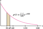
Solution If the average waiting time is \(60\) seconds, then \(r = 60\) and \(p(t) = \frac{1}{60} e^{-t/60}\) because the mean of \(p(t)\) is \(r\) by the previous example. Therefore, the probability of waiting between \(30\) and \(45\) seconds for the next customer is \[ P(30\le T\le 45) = \int_{30}^{45}\frac1{60}e^{-t/60} = -e^{-t/60}\Big|_{30}^{45} = -e^{-3/4}+e^{-1/2}\approx 0.134 \]
This probability is the area of the shaded region in Figure 7.19.
The normal density functions, whose graphs are the familiar bell-shaped curves, appear in a surprisingly wide range of applications. The standard normal density is defined by \[ \boxed{\bbox[#FAF8ED,5pt]{p(x) = \frac1{\sqrt{2\pi}}\,e^{-x^2/2}}}\tag{3} \]
We can prove that \(p(x)\) satisfies Eq. (1) using multivariable calculus.
450
More generally, we define the normal density function with mean \(\mu\) and standard deviation \(\sigma\): \[ \boxed{\bbox[#FAF8ED,5pt]{ p(x) = \frac1{\sigma\sqrt{2\pi}}\,e^{-(x-\mu)^2/(2\sigma^2)}} }\]
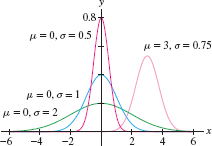
The standard deviation \(\sigma\) measures the spread; for larger values of \(\sigma\) the graph is more spread out about the mean \(\mu\) (Figure 7.20). The standard normal density in Eq. (3) has mean \(\mu=0\) and \(\sigma = 1\). A random variable with a normal density function is said to have a normal or Gaussian distribution.
One difficulty is that normal density functions do not have elementary antiderivatives. As a result, we cannot evaluate the probabilities \[ P(a \le X \le b) = \frac1{\sigma\sqrt{2\pi}}\int_a^b\,e^{-(x-\mu)^2/(2\sigma^2)}\,dx \]
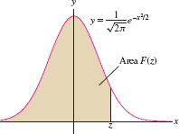
explicitly. However, the next theorem shows that these probabilities can all be expressed in terms of a single function called the standard normal cumulative distribution function: \[ \boxed{\bbox[#FAF8ED,5pt]{ F(z) = \frac1{\sqrt{2\pi}}\int_{-\infty}^z\, \,e^{-x^2/2}\,dx }}\]
Observe that \(F(z)\) is equal to the area under the graph over \((-\infty,z]\) in Figure 7.21. Numerical values of \(F(z)\) are widely available on scientific calculators, on computer algebra systems, and online (search “standard cumulative normal distribution”).
THEOREM 1
If \(X\) has a normal distribution with mean \(\mu\) and standard deviation \(\sigma\), then for all \(a\le b\), \[ \boxed{\bbox[#FAF8ED,5pt]{P( X\le b) = F\left(\frac{b-\mu}{\sigma}\right)}}\tag{4} \] \[\boxed{\bbox[#FAF8ED,5pt]{ P(a\le X\le b) = F\left(\frac{b-\mu}{\sigma}\right) - F\left(\frac{a-\mu}{\sigma}\right)}}\tag{5} \]
Proof
We use two changes of variables, first \(u=x-\mu\) and then \(t = u/\sigma\): \[ \begin{align*} P(X\le b) &= \frac1{\sigma\sqrt{2\pi}}\int_{-\infty}^b\,e^{-(x-\mu)^2/(2\sigma^2)}\,dx = \frac1{\sigma\sqrt{2\pi}}\int_{-\infty}^{b-\mu}\,e^{-u^2/(2\sigma^2)}\,du\\ &=\frac1{\sqrt{2\pi}} \int_{-\infty}^{(b-\mu)/\sigma}\,e^{-t^2/2}\,dt = F\left(\frac{b-\mu}{\sigma}\right) \end{align*} \]
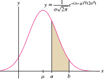
This proves Eq. (4). Eq. (5) follows because \(P(a\le X\le b)\) is the area under the graph between \(a\) and \(b\), and this is equal to the area to the left of \(b\) minus the area to the left of \(a\) (Figure 7.22).
451
EXAMPLE 4
Assume that the scores \(X\) on a standardized test are normally distributed with mean \(\mu=500\) and standard deviation \(\sigma = 100\). Find the probability that a test chosen at random has score
- at most 600.
- between 450 and 650.
Solution We use a computer algebra system to evaluate \(F(z)\) numerically.
- Apply Eq. (4) with \(\mu = 500\) and \(\sigma = 100\):
\[
P(x\le 600) = F\left(\frac{600-500}{100}\right) = F(1)\approx 0.84
\]
Thus, a randomly chosen score is \(600\) or less with a probability of \(0.84\), or \(84\%\).
- Applying Eq. (5), we find that a randomly chosen score lies between \(450\) and \(650\) with a probability of \(62.5\%\): \[ P(450 \le x\le 650) = F(1.5)-F(-0.5)\approx 0.933 - 0.308 = 0.625 \]
CONCEPTUAL INSIGHT
Why have we defined the mean of a continuous random variable \(X\) as the integral \(\mu=\int_{-\infty}^\infty xp(x)\,dx\)?
Suppose first we are given \(N\) numbers \(a_1, a_2, \ldots, a_N\), and for each value \(x\), let \(N(x)\) be the number of times \(x\) occurs among the \(a_j\). Then a randomly chosen \(a_j\) has value \(x\) with probability \(p(x) = N(x)/N\). For example, given the numbers \(4, 4, 5, 5, 5, 8\), we have \(N=6\) and \(N(5) = 3\). The probability of choosing a \(5\) is \(p(5)=N(5)/N=\frac36=\frac12\). Now observe that we can write the mean (average value) of the \(a_j\) in terms of the probabilities \(p(x)\): \[ \frac{a_1 + a_2 + \cdots + a_N}N = \frac1N \sum_{x}\, N(x)x = \sum_{x}\, xp(x) \]
For example, \[ \frac{4+4+5+5+5+8}6 = \frac16\left(2\cdot 4 + 3\cdot 5 + 1\cdot 8\right)= 4p(4)+5p(5)+8p(8) \]
In defining the mean of a continuous random variable \(X\), we replace the sum \({\sum_{x}xp(x)}\) with the integral \(\mu = \int_{-\infty}^\infty xp(x)\,dx\). This makes sense because the integral is the limit of sums \({\sum x_ip(x_i)\Delta x}\), and as we have seen, \(p(x_i)\Delta x\) is the approximate probability that \(X\) lies in \([x_i,x_i+\Delta x]\).
7.7.1 Summary
- If \(X\) is a continuous random variable with probability density function \(p(x)\), then \[ P(a\le X \le b) = \int_a^b\,p(x)\, dx \]
- Probability densities satisfy two conditions: \(p(x)\ge 0\) and
\(\int_{-\infty}^\infty \,p(x)\,dx=1\).
452
- Mean (or average) value of \(X\): \[{ \mu = \int_{-\infty}^\infty xp(x)\,dx}\]
- Exponential density function of mean \(r\): \[p(x) = \frac1r\,e^{-x/r}\]
- Normal density of mean \(\mu\) and standard deviation \(\sigma\): \[ p(x) = \frac1{\sigma\sqrt{2\pi}} \,e^{-(x-\mu)^2/(2\sigma^2)} \]
- Standard cumulative normal distribution function: \[ F(z) = \frac1{\sqrt{2\pi}}\int_{-\infty}^z\, \,e^{-t^2/2}\,dt \]
- If \(X\) has a normal distribution of mean \(\mu\) and standard deviation \(\sigma\), then \[ \begin{align*} P(X\le b) &= F\left(\frac{b-\mu}{\sigma}\right) \\ P(a\le X\le b) &= F\left(\frac{b-\mu}{\sigma}\right) - F\left(\frac{a-\mu}{\sigma}\right) \end{align*} \]