18.4 Gauss’ Theorem
Gauss’ theorem states that the flux of a vector field out of a closed surface equals the integral of the divergence of that vector field over the volume enclosed by the surface. The result parallels Stokes’ theorem and Green’s theorem in that it relates an integral over a closed geometric object (curve or surface) to an integral over a contained region (surface or volume).
Elementary Regions and Their Boundaries
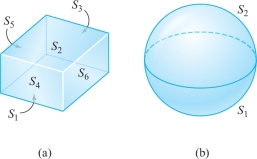
We shall begin by asking you to review the various elementary regions in space that were introduced when we considered the volume integral; these regions are illustrated in Figures 15.31 and 15.33 As these figures indicate, the boundary of an elementary region in \({\mathbb R}^3\) is a surface made up of a finite number (at most six, at least two) of surfaces that can be described as graphs of functions from \({\mathbb R}^2\) to \({\mathbb R}\). This kind of surface is called a closed surface. The surfaces \(S_1 , S_2, \ldots , S_N\) composing such a closed surface are called its faces.
example 1
The cube in Figure 18.30(a) is an elementary region, and in fact a symmetric elementary region, with six rectangles composing its boundary. The sphere in Figure 18.30(b) is the boundary of a solid ball, which is also a symmetric elementary region.
462
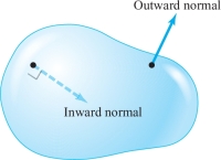
Closed surfaces can be oriented in two ways. The outward orientation makes the normal point outward into space, and the inward orientation makes the normal point into the bounded region (Figure 18.31).
Suppose \(S\) is a closed surface oriented in one of these two ways and \({\bf F}\) is a vector field on \(S\). Then, as we defined it in Section 7.6, \[ \intop\!\!\!\intop\nolimits_{S} {\bf F} \,{\cdot}\, d {\bf S} = \sum_i \intop\!\!\!\intop\nolimits_{S_i} {\bf F} \,{\cdot}\, d {\bf S}. \]
If \(S\) is given the outward orientation, the integral \({\intop\!\!\!\intop}_S {\bf F} \,{\cdot}\, d {\bf S}\) measures the total flux of \({\bf F}\) outward across \(S\). That is, if we think of \({\bf F}\) as the velocity field of a fluid, \({\intop\!\!\!\intop}_S {\bf F} \,{\cdot}\, d {\bf S}\) indicates the amount of fluid leaving the region bounded by \(S\) per unit time. If \(S\) is given the inward orientation, the integral \({\intop\!\!\!\intop}_S {\bf F} \,{\cdot}\, d {\bf S}\) measures the total flux of \({\bf F}\) inward across \(S\).
We recall another common way of writing these surface integrals, a way that explicitly specifies the orientation of \(S\). Let the orientation of \(S\) be given by a unit normal vector \({\bf n} (x,y,z)\) at each point of \(S\). Then we have the oriented integral \[ \intop\!\!\!\intop\nolimits_{S} {\bf F} \,{\cdot}\, d {\bf S} = \intop\!\!\!\intop\nolimits_{S} ( {\bf F} \,{\cdot}\, {\bf n} )\ d S, \] that is, the integral of the normal component of \({\bf F}\) over \(S\). In the remainder of this section, if \(S\) is a closed surface enclosing a region \(W\), we adopt the default convention that \(S= \partial\! W\) is given the outward orientation, with outward unit normal \({\bf n} (x,y,z)\) at each point \((x,y,z) \in S\). Furthermore, we denote the surface with the opposite (inward) orientation by \(\partial\! W_{\rm op}\). Then the associated unit normal direction for this orientation is \(- {\bf n}\). Thus, \[ \intop\!\!\!\intop\nolimits_{\partial\! W} {\bf F} \,{\cdot}\, d {\bf S} = \intop\!\!\!\intop\nolimits_{S} ( {\bf F} \,{\cdot}\, {\bf n}) {\,d} S =- \intop\!\!\!\intop\nolimits_{S} [ {\bf F} \,{\cdot}\, (-{\bf n} ) ] {\,d} S =- \intop\!\!\!\intop\nolimits_{\partial\! W_{\rm op}} {\bf F} \,{\cdot}\, d {\bf S}. \]
example 2
The unit cube \(W\) given by \[ 0 \le x \le 1, \qquad 0 \le y \le 1, \qquad 0 \le z \le 1 \] is a symmetric elementary region in space (see Figure 18.32 and Figure 15.34).
We write the faces as \begin{eqnarray*} S_1 \colon\, z &=& 0, \qquad 0 \le x \le 1, \qquad 0 \le y \le 1 \\ S_2 \colon\, z &=&1, \qquad 0 \le x \le 1, \qquad 0 \le y \le 1 \\ S_3 \colon\, x &=&0, \qquad 0 \le y \le 1, \qquad 0 \le z \le 1 \\ S_4 \colon\, x &=&1, \qquad 0 \le y \le 1, \qquad 0 \le z \le 1 \\ S_5 \colon\, y &=&0, \qquad 0 \le x \le 1, \qquad 0 \le z \le 1 \\ S_6 \colon\, y &=&1, \qquad 0 \le x \le 1, \qquad 0 \le z \le 1. \\[-36pt] \end{eqnarray*}
463
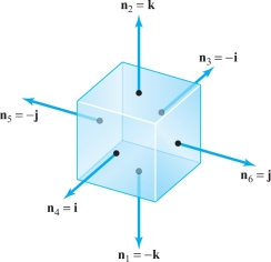
From Figure 18.32, we see that \begin{eqnarray*} && {\bf n}_2 = {\bf k} = - {\bf n}_1 , \\ && {\bf n}_4 = {\bf i} = - {\bf n}_3 , \\ && {\bf n}_6 = {\bf j} = - {\bf n}_5 , \end{eqnarray*} and so for a continuous vector field \({\bf F} = F_1 {\bf i} + F_2 {\bf j} + F_3 {\bf k}\), \begin{eqnarray*} \intop\!\!\!\intop\nolimits_{\partial\! W} {\bf F} \,{\cdot}\, d {\bf S} &=& \intop\!\!\!\intop\nolimits_{S} {\bf F} \,{\cdot}\, {\bf n} {\,d} S = - \intop\!\!\!\intop\nolimits_{S_1} F_3\, dS + \intop\!\!\!\intop\nolimits_{S_2} F_3\, d S - \intop\!\!\!\intop\nolimits_{S_3} F_1 {\,d} S \\[5pt] && + \intop\!\!\!\intop\nolimits_{S_4} F_1 {\,d} S - \intop\!\!\!\intop\nolimits_{S_5} F_2 {\,d} S + \intop\!\!\!\intop\nolimits_{S_6} F_2 {\,d} S.\\[-28pt] \end{eqnarray*}
Gauss’ Theorem
We have now come to the last of the three central theorems of this chapter. This theorem relates surface integrals to volume integrals; in other words, the theorem states that if \(W\) is a region in \({\mathbb R}^3\), then the flux of a vector field \({\bf F}\) outward across the closed surface \(\partial\! W\) is equal to the integral of div \({\bf F}\) over \(W\). We begin by assuming that \(W\) is a symmetric elementary region (Figure 15.34).
Theorem 9 Gauss’ Divergence Theorem
Let \(W\) be a symmetric elementary region in space. Denote by \(\partial\! W\) the oriented closed surface that bounds \(W\). Let \({\bf F}\) be a smooth vector field defined on \(W\). Then \[ \intop\!\!\!\intop\!\!\!\intop\nolimits_{W} ({\nabla} \,{\cdot}\, {\bf F} ) {\,d} V = \intop\!\!\!\intop\nolimits_{\partial\! W} {\bf F} \,{\cdot}\, d {\bf S} \] or, alternatively, \[ \intop\!\!\!\intop\!\!\!\intop\nolimits_{W} ({\rm div\ } {\bf F}) {\,d} V = \intop\!\!\!\intop\nolimits_{\partial\! W} ( {\bf F} \,{\cdot}\, {\bf n}) {\,d} S. \]
464
proof
If \({\bf F} = P {\bf i} + Q {\bf j} + R {\bf k}\), then by definition, the divergence of \({\bf F}\) is given by div \({\bf F} = \partial\! P / \partial x + \partial\! Q / \partial y + \partial\! R/\partial z\), so we can write (using additivity of the volume integral) \[ \intop\!\!\!\intop\!\!\!\intop\nolimits_{W} \hbox{div } {\bf F} {\,d} V = \intop\!\!\!\intop\!\!\!\intop\nolimits_{W} \frac{\partial\! P}{\partial x} {\,d} V + \intop\!\!\!\intop\!\!\!\intop\nolimits_{W} \frac{\partial\! Q}{\partial y} {\,d} V + \intop\!\!\!\intop\!\!\!\intop\nolimits_{W} \frac{\partial\! R}{ \partial z} {\,d} V. \]
On the other hand, the surface integral in question is \begin{eqnarray*} \intop\!\!\!\intop\nolimits_{\partial\! W} {\bf F} \,{\cdot}\, {\bf n} {\,d} S &=& \intop\!\!\!\intop\nolimits_{\partial\! W}(P{\bf i}+Q{\bf j} +R{\bf k})\,{\cdot}\,{\bf n}{\,d} S\\[6pt] &=& \intop\!\!\!\intop\nolimits_{\partial\! W} P {\bf i} \,{\cdot}\, {\bf n} {\,d} S + \intop\!\!\!\intop\nolimits_{\partial\! W} Q {\bf j} \,{\cdot}\, {\bf n}{\,d} S + \intop\!\!\!\intop\nolimits_{\partial\! W} R {\bf k} \,{\cdot}\, {\bf n} {\,d} S.\\[-16pt] \end{eqnarray*}
The theorem will follow if we establish the three equalities \begin{equation*} \intop\!\!\!\intop\nolimits_{\partial\! W} P {\bf i} \,{\cdot}\, {\bf n} {\,d} S = \intop\!\!\!\intop\!\!\!\intop\nolimits_{W} \frac{\partial\! P}{\partial x} {\,d} V, \tag{1} \end{equation*} \begin{equation*} \intop\!\!\!\intop\nolimits_{\partial\! W} Q {\bf j} \,{\cdot}\, {\bf n} {\,d} S = \intop\!\!\!\intop\!\!\!\intop\nolimits_{W} \frac{\partial\! Q}{\partial y} {\,d} V,\tag{2} \end{equation*} and \begin{equation*} \intop\!\!\!\intop\nolimits_{\partial\! W} R {\bf k} \,{\cdot}\, {\bf n} {\,d} S = \intop\!\!\!\intop\!\!\!\intop\nolimits_{W} \frac{\partial\! R}{\partial z} {\,d} V.\tag{3} \end{equation*}
We shall prove equation (3); the other two equalities can be proved in an analogous fashion.
Because \(W\) is a symmetric elementary region, there is a pair of functions \[ z =g_1 (x,y) ,\qquad z = g_2 (x,y), \] with common domain an elementary region \(D\) in the \(xy\) plane, such that \(W\) is the set of all points \((x,y,z)\) satisfying \[ g_1 (x,y) \le z \le g_2 (x,y), \qquad (x,y) \in D. \]
By reduction to iterated integrals, we have \[ \intop\!\!\!\intop\!\!\!\intop\nolimits_{W} \frac{\partial\! R}{\partial z} {\,d} V = \intop\!\!\!\intop\nolimits_{D} \left( \int_{z=g_1(x,y)}^{z=g_2(x,y)} \frac{\partial\! R}{\partial z} {\,d} z \right) {\it dx}\, {\it dy}, \] and so, by the fundamental theorem of calculus, \begin{equation*} \intop\!\!\!\intop\!\!\!\intop\nolimits_{W} \frac{\partial\! R}{\partial z} {\,d} V = \intop\!\!\!\intop\nolimits_{D} [R (x,y,g_2 (x,y)) - R (x,y,g_1 (x,y))] {\it {\,d} x}\, {\it dy}.\tag{4} \end{equation*}
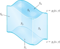
The boundary of \(W\) is a closed surface whose top \(S_2\) is the graph of \(z= g_2 (x,y)\), where \((x,y) \in D\), and whose bottom \(S_1\) is the graph of \(z= g_1 (x,y), (x,y) \in D\). The four other sides of \(\partial\! W\) consist of surfaces \(S_3, S_4, S_5\), and \(S_6\), whose normals are always perpendicular to the \(z\) axis. (See Figure 18.33. Note that some of the other four sides might be absent; for instance, if \(W\) is a solid ball and \(\partial\! W\) is a sphere.) By definition, \[ \intop\!\!\!\intop\nolimits_{\partial\! W} R {\bf k} \,{\cdot}\, {\bf n} {\,d} S = \intop\!\!\!\intop\nolimits_{S_1} R {\bf k} \,{\cdot}\, {\bf n}_1 {\,d} S + \intop\!\!\!\intop\nolimits_{S_2} R {\bf k} \,{\cdot}\, {\bf n}_2 {\,d} S + \sum_{i=3}^6 \intop\!\!\!\intop\nolimits_{S_i} R {\bf k} \,{\cdot}\, {\bf n}_i {\,d} S. \]
465
Because the normal \({\bf n}_{i}\) is perpendicular to \({\bf k}\) on each of \(S_{3}, S_{4}, S_{5}, S_{6}\), we have \({\bf k}\, {\cdot}\, {\bf n} = 0\) along these faces, and so the integral reduces to \begin{equation*} \intop\!\!\!\intop\nolimits_{\partial\! W} R {\bf k} \,{\cdot}\, {\bf n} {\,d} s = \intop\!\!\!\intop\nolimits_{S_1} R {\bf k} \,{\cdot}\, {\,d} {\bf S}_1 + \intop\!\!\!\intop\nolimits_{S_2} R {\bf k} \,{\cdot}\, {\,d} {\bf S}_2.\tag{5} \end{equation*}
The surface \(S_1\) is defined by \(z=g_1(x,y)\), and \[ d{\bf S}_1 = \left(\frac{\partial g_1}{\partial x}{\bf i} + \frac{\partial g_1}{\partial y}{\bf j}- {\bf k} \right)\!\! {\it {\,d} x}\, {\it dy} \] (the negative of the general formula for \(d{\bf S}\) for graphs from Section 7.6, because the normal is downward pointing). Therefore, \begin{equation*} \intop\!\!\!\intop\nolimits_{S_1} R{\bf k}\, {\cdot}\, d{\bf S}_1 = - \intop\!\!\!\intop\nolimits_D R (x,y, g_1 (x, y))\, {\it {\,d} x}\, {\it dy}.\tag{6} \end{equation*}
Similarly, for the top face \(S_{2}\), \[ d{\bf S}_2 = \left(-\frac{\partial g_2}{\partial x}{\bf i} -\frac{\partial g_2}{\partial y}{\bf j} + {\bf k} \right)\!\!{\it {\,d} x}\, {\it dy}. \]
Therefore, \begin{equation*} \intop\!\!\!\intop\nolimits_{S_2} R{\bf k} \,{\cdot}\, d{\bf S}_2 = \intop\!\!\!\intop\nolimits_D R(x, y, g_2 (x, y))\, {\it {\,d} x}\, {\it dy}.\tag{7} \end{equation*}
Substituting equations (6) and (7) into equation (5) and then comparing with equation (4), we obtain \[ \intop\!\!\!\intop\!\!\!\intop\nolimits_{W} \frac{\partial\! R}{\partial z} {\,d} V = \intop\!\!\!\intop\nolimits_{\partial\! W} R ( {\bf k} \,{\cdot}\, {\bf n}) {\it {\,d} S}. \]
The remaining equalities, (1) and (2), can be established in the same way to complete the proof.
Generalizing Gauss’ Theorem
466
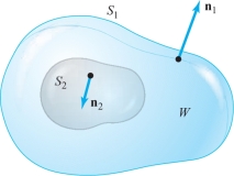
The reader should note that the proof of Gauss’ theorem is similar to that of Green’s theorem. By the procedure used in Exercise 16 of Section 18.1, we can extend Gauss’ theorem to any region that can be broken up into symmetric elementary regions. This includes all regions of interest to us. An example of a region to which Gauss’ theorem applies is the region between two closed surfaces, one inside the other. The surface of this region consists of two pieces oriented as shown in Figure 18.34. We shall apply the divergence theorem to such a region when we prove Gauss’ law in Theorem 10.
example 3
Consider \({\bf F} = 2 x {\bf i} + y^2 {\bf j}+ z^2 {\bf k}\). Let \(S\) be the unit sphere defined by \(x^2 + y^2 + z^2 =1\). Evaluate \({\intop\!\!\!\intop}_S {\bf F} \,{\cdot}\, {\bf n} \,\,{\,d} S\).
solution By Gauss’ theorem, \[ \intop\!\!\!\intop\nolimits_{S} {\bf F} \,{\cdot}\, {\bf n} {\,d} S= \intop\!\!\!\intop\!\!\!\intop\nolimits_{W} (\hbox{div } {\bf F} ) {\,d} V , \] where \(W\) is the ball bounded by the sphere. The integral on the right is \[ 2 \intop\!\!\!\intop\!\!\!\intop\nolimits_{W} (1+ y+ z) {\,d} V = 2 \intop\!\!\!\intop\!\!\!\intop\nolimits_{W} {\,d} V +2 \intop\!\!\!\intop\!\!\!\intop\nolimits_{W} y{\,d} V + 2 \intop\!\!\!\intop\!\!\!\intop\nolimits_{W} z {\,d} V. \]
By symmetry, we can argue that \({\intop\!\!\!\intop\!\!\!\intop}_W y {\,d} V = {\intop\!\!\!\intop\!\!\!\intop}_W z {\,d} V =0\) (see Exercise 21, Section 6.3). Thus, because a sphere of radius \(R\) has volume \(4\pi R^3/3\), \[ 2 \intop\!\!\!\intop\!\!\!\intop\nolimits_{W} (1+ y +z) {\,d} V = 2 \intop\!\!\!\intop\!\!\!\intop\nolimits_{W} {\,d} V = \frac{8 \pi}{3}. \]
You can convince yourself that direct computation of \({\intop\!\!\!\intop}_S {\bf F} \,{\cdot}\, {\bf n} \,dS\) proves unwieldy.
Question 18.111 Section 18.4 Progress Check Question #1
Bt1YnzjJbyNUPzMH1NgWLZk0YDLsif9AqZpgiU6kLhovk1J6kKE9IMiMnaTc3qPuLUca2Ua7ViNn+c1qIgBtZG0ayawTFJS6W3mikxhQe0PWhUBATQuq1FEzBv+oFDpX3yQ1D1BvUCziHrbqtNpJDREALDa4xPyqHTwP/P9Z3NLftJRBkgcvokY5Ur4SrYpF7MoV7OWmd0uokmYoiCtZKorznz2/yDlEWpiOSijBBY89cBrr2wWnBXY8ZAFpUF0nfPPcQU5JJMiPxXIwKZXDP0FJTa4F5c4iAeyuC8EhT27OwTCM9JjTUkU9QnzqOBwtt9kGtRm3htfNksE2WWhe3JSNrYY94CO/rRxuJ0tnKszhRH65YeM9aQSnC2uWPZ/K0EGHihhGWEZTF6W/x62qt5giSwW/LxE1MW/RU5wTl6wzUov2zV8J5kFERvw=example 4
Use the divergence theorem to evaluate \[ \intop\!\!\!\intop\nolimits_{\partial\! W} (x^2 + y +z ) {\,d} S, \] where \(W\) is the solid ball \(x^2 +y^2 + z^2 \le 1\).
467
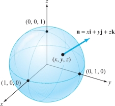
solution To apply Gauss’ divergence theorem, we find a vector field \({\bf F} = F_1 {\bf i} + F_2 {\bf j} + F_3 {\bf k}\) on \(W\) with \({\bf F} \,{\cdot}\, {\bf n} = x^2 + y +z\). At any point \((x,y,z) \in \partial\! W\), the outward unit normal \({\bf n}\) to \(\partial\! W\) is \[ {\bf n} = x {\bf i} + y {\bf j}+ z {\bf k}, \] because on \(\partial\! W, x^2 + y^2 + z^2=1\) and the radius vector \({\bf r} = x {\bf i} + y {\bf j} + z {\bf k}\) is normal to the sphere \(\partial\! W\) (Figure 18.35).
Therefore, if \({\bf F}\) is the desired vector field, then \[ {\bf F} \,{\cdot}\, {\bf n} = F_1 x + F_2 y + F_2 z. \]
We set \[ F_1 x = x^2, \qquad F_2 y =y, \qquad F_3 z=z \] and solve for \(F_1,F_2\), and \(F_3\) to find that \({\bf F} = x {\bf i} + {\bf j} + {\bf k}\). Computing div \({\bf F}\), we get \[ \hbox{div } {\bf F} = 1+ 0 + 0 =1. \]
Thus, by Gauss’ divergence theorem, \[ \intop\!\!\!\intop\nolimits_{\partial\! W} (x^2 + y + z ) {\,d} S = \intop\!\!\!\intop\!\!\!\intop\nolimits_{W} {\,d} V = \hbox{volume } (W) = \frac{4}{3} \pi. \]
The Divergence as the Flux per Unit Volume
The physical meaning of divergence is that at a point P, div \({\bf F}\)(P) is the rate of net outward flux at P per unit volume. This follows from Gauss’ theorem and the mean-value theorem for integrals: If \(W_{\rho}\) is a ball in \({\mathbb R}^3\) of radius \(\rho\) centered at P, then there is a point \({\rm Q}\in W_{\rho}\) such that \[ \intop\!\!\!\intop\nolimits_{\partial\! W_{\rho}}{\bf F}\,{\cdot}\,{\bf n}{\,d} S= \intop\!\!\!\intop\!\!\!\intop\nolimits_{W_{\rho}}\hbox{div }{\bf F}{\,d} V=\hbox{div }{\bf F}({\rm Q})\,{\cdot}\, \hbox{volume }(W_\rho) \] and so \[ \hbox{div }{\bf F}({\rm P})=\mathop{\rm limit}_{\rho\to 0}\hbox{div }{\bf F}({\rm Q})=\mathop{\rm limit}_{\rho\to 0}\frac{1}{V(W_{\rho})}\intop\!\!\!\intop\nolimits_{\partial\! W_{\rho}}{\bf F}\,{\cdot}\,{\bf n}{\,d} S. \]
468
This is analogous to the limit formulation of the curl given at the end of Section 18.2. Thus, if div \({\bf F}{\rm (P)} >0\), we consider P to be a source, for there is a net outward flow near P. If div \({\bf F}{\rm (P)}<0\), P is called a sink for \({\bf F}\).
A \(C^1\) vector field \({\bf F}\) defined on \({\mathbb R}^3\) is said to be divergence-free if div \({\bf F}=0\). If \({\bf F}\) is divergence-free, we have \({\intop\!\!\!\intop}_S{\bf F}\,{\cdot}\,{\,d} {\bf S}=0\) for all closed surfaces \(S\). The converse can also be demonstrated readily using Gauss’ theorem: If \({\intop\!\!\!\intop}_S{\bf F}\,{\cdot}\,{\,d} {\bf S}=0\) for all closed surfaces \(S\), then \({\bf F}\) is divergence-free. If \({\bf F}\) is divergence-free, we thus see that the flux of \({\bf F}\) across any closed surface \(S\) is 0, so that if \({\bf F}\) is the velocity field of a fluid, the net amount of fluid that flows out of any region will be 0. Thus, exactly as much fluid must flow into the region as flows out (in unit time). A fluid with this property is therefore described as incompressible.
example 5
Evaluate \({\intop\!\!\!\intop}_S{\bf F}\,{\cdot}\,{\,d} {\bf S}\), where \({\bf F}(x,y,z)=xy^2{\bf i}\,+\,x^2y {\bf j}\,+\,y{\bf k}\) and \(S\) is the surface of the cylinder \(x^2+y^2=1\), bounded by the planes \(z=1\) and \(z=-1\), and including the portions \(x^2+y^2\leq 1\) when \(z=\pm 1\).
solution We can compute this integral directly, but it is easier to use the divergence theorem.
Now \(S\) is the boundary of the region \(W\) given by \(x^2+y^2\leq 1,-1\leq z\leq 1\). Thus, \({\intop\!\!\!\intop}_S{\bf F}\,{\cdot}\,{\,d} {\bf S}={\intop\!\!\!\intop\!\!\!\intop}_W(\hbox{div } {\bf F}) {\,d} V\). Moreover, \begin{eqnarray*} \intop\!\!\!\intop\!\!\!\intop\nolimits_{W}(\hbox{div } {\bf F}){\,d} V=\intop\!\!\!\intop\!\!\!\intop\nolimits_{W}(x^2+y^2)\,{\it {\,d} x}\,{\it dy}\,{\,d} z &=& \int_{-1}^1\left(\int_{x^2+y^2\leq 1}(x^2+y^2)\,{\it {\,d} x}\,{\it dy}\right)\!\!{\,d} z\\[6pt] &=& 2\intop\!\!\!\intop\nolimits_{x^2+y^2\leq 1}(x^2+y^2)\,{\it {\,d} x}\,{\it dy}. \end{eqnarray*}
Before evaluating the double integral, we note that the surface integral satisfies \[ \intop\!\!\!\intop\nolimits_{\partial\! W}{\bf F}\,{\cdot}\, {\bf n}{\,d} S=2\intop\!\!\!\intop\nolimits_{x^2+y^2\leq 1}(x^2+y^2)\,{\it {\,d} x}\,{\it dy}>0. \]
This means that \({\intop\!\!\!\intop}_{\partial\! W}{\bf F}\,{\cdot}\,{\,d} {\bf S}\), the net flux of \({\bf F}\) out of the cylinder, is positive.
We change variables to polar coordinates to evaluate the double integral: \[ x=r\cos\theta,\qquad y=r\sin\theta,\qquad 0\leq r \leq 1,\qquad 0\leq \theta\leq 2\pi. \]
Hence, we have \(\partial (x,y)/\partial (r,\theta)=r\) and \(x^2+y^2=r^2\). Thus, \[ \intop\!\!\!\intop\nolimits_{x^2+y^2\leq 1}(x^2+y^2)\,{\it {\,d} x}\,{\it dy}=\int_0^{2\pi} \left(\int_0^1 r^3{\,d} r\right)\!\!{\,d}\theta=\frac{1}{2}\pi. \]
Therefore, \({\intop\!\!\!\intop\!\!\!\intop}_W\hbox{div }{\bf F}{\,d} V=\pi\).
Question 18.112 Section 18.4 Progress Check Question #2
OL7NEzcYEdmuc52UTHmnZl1du0d4zpYz1so8uVPRcX8UDYGRKMivEUspO1zDkTsofbiwhN/ncyGHdNV42TW8PEadDL9D3YaNOaboD3QEqvxcyteF07A2FpRwwiRCKBxNRo42luGEQnnkgGuuifWD9YioGgho4T9S3YL7pfICzxF4OMHBSBOiVIEODxU+e6CCt9IN62SJmRW096ayYJbGQd8EnlpwfhJJDGpYeI9WG/7BIYWFVay4y8ZmopdaqKB4z6facc6vVyWNs73Fs9Je2BfnOlYrPReoB5wRiwIvXVTS5Ylco84/f+tr43CwvZAed6/dxLQtcNgbJ4yN/+mAsM+lajwyRiMp4sRldtx5fA6azyfpW+yeaZm8VVtApvXx8wJv2yPRUd3OvycKTYxVer757PfzqT47AcYf/j/UgO/+K258J+DZsF9rwCMHeaADGG0U5Fg7AE34SH0qojX8Z720ANXsccu/ZgixIKqZSFiqe0WemFQnxJbtyTKqEzidexTTgNgBHBAm24EvSbZ0n/QGscjKj7IHK1aGtGZJK+IsjAfJlScu/twRr0E7FEyOzgfKsCa1veRnn/hq8CTRxsxu3aT3yuBosqNIs8yPb9k=Gauss’ Law
As we remarked earlier, Gauss’ divergence theorem can be applied to regions in space more general than symmetric elementary regions. To conclude this section, we shall use this observation in the proof of the following important results.
469
Theorem 10 Gauss’ Law
Let \(M\) be a symmetric elementary region in \({\mathbb R}^3\). Then if \((0, 0, 0){\not\in} \,\partial\! M\), we have \[ \intop\!\!\!\intop\nolimits_{\partial\! M}\frac{{\bf r}\,{\cdot}\, {\bf n}}{r^3} {\,d} S= \bigg\{ \begin{array}{l@{\qquad}l} 4\pi & \hbox{if }\, (0,0,0)\in M\\ 0 & \hbox{if }\, (0,0,0){\not\in}\, M, \end{array} \] where \[ {\bf r}(x,y,z)=x{\bf i}+y{\bf j}+z{\bf k} \] and \[ r(x,y,z) =\|{\bf r}(x,y,z)\|={\textstyle\sqrt{x^2+y^2+z^2}}. \]
proof of Gauss’ law
First suppose \((0, 0, 0)\,{\not\in}\, M\). Then \({\bf r}/r^3\) is a \(C^1\) vector field on \(M\) and \(\partial\! M\), and so by the divergence theorem, \[ \intop\!\!\!\intop\nolimits_{\partial\! M}\frac{{\bf r}\,{\cdot}\, {\bf n}}{r^3}{\,d} S=\intop\!\!\!\intop\!\!\!\intop\nolimits_{M} {\nabla}\,{\cdot}\, \left(\frac{{\bf r}}{r^3}\right){\,d} V. \]
But \({\nabla}\,{\cdot}\,({\bf r}/r^3)=0\) for \(r\neq 0\), as you can easily verify (see Exercise 38, Section 4.4). Thus, \[ \intop\!\!\!\intop\nolimits_{\partial\! M}\frac{{\bf r}\,{\cdot}\, {\bf n}}{r^3}{\,d} S=0. \]
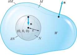
Now let us suppose \((0, 0, 0)\in M\). We can no longer use the preceding method, because \({\bf r}/r^3\) is not smooth on \(M\), due to the zero denominator at \({\bf r}=(0,0,0)\). Because \((0,0,0)\in M\) and \((0,0,0){\not\in} \partial\! M\), there is an \(\varepsilon > 0\) such that the ball \(N\) of radius \(\varepsilon\) centered at (0, 0, 0) is contained completely inside \(M\). Let \(W\) be the region between \(M\) and \(N\). Then \(W\) has boundary \(\partial\! N\cup \partial\! M=S\). But the orientation on \(\partial\! N\) induced by the outward normal on \(W\) is the opposite of that obtained from \(N\) (see Figure 18.36).
Now \({\nabla}\,{\cdot}\,({\bf r}/r^3)=0\) on \(W\), and so, by the divergence theorem applied to the (nonelementary) region \(W\), \[ \intop\!\!\!\intop\nolimits_{S}\frac{{\bf r}\,{\cdot}\, {\bf n}}{r^3} {\,d} S= \intop\!\!\!\intop\!\!\!\intop\nolimits_{W}{\nabla}\,{\cdot}\, \left(\frac{{\bf r}}{r^3}\right) dV=0. \]
470
Because \[ \intop\!\!\!\intop\nolimits_{S}\frac{{\bf r}\,{\cdot}\, {\bf n}}{r^3} {\,d} S =\intop\!\!\!\intop\nolimits_{\partial\! M} \frac{{\bf r}\,{\cdot}\, {\bf n}}{r^3} {\,d} S +\intop\!\!\!\intop\nolimits_{\partial\! N} \frac{{\bf r}\,{\cdot}\, {\bf n}}{r^3} {\,d} S, \] where \({\bf n}\) is the outward normal to \(S\), we have \[ \intop\!\!\!\intop\nolimits_{\partial\! M}\frac{{\bf r}\,{\cdot}\, {\bf n}}{r^3}{\,d} S=-\intop\!\!\!\intop\nolimits_{\partial\! N}\frac{{\bf r}\,{\cdot}\, {\bf n}}{r^3} {\,d} S. \]
However, on \(\partial\! N, {\bf n}=-{\bf r}/r\) and \(r=\varepsilon\), because \(\partial\! N\) is a sphere of radius \(\varepsilon\), so that \[ -\intop\!\!\!\intop\nolimits_{\partial\! N}\frac{{\bf r}\,{\cdot}\, {\bf n}}{r^3} {\,d} S=\intop\!\!\!\intop\nolimits_{\partial\! N} \frac{\varepsilon^2}{\varepsilon^4}{\,d} S= \frac{1}{\varepsilon^2}\intop\!\!\!\intop\nolimits_{\partial\! N}{\,d} S. \]
But \({\intop\!\!\!\intop}_{\partial\! N}{\,d} S=4\pi\varepsilon^2\), the surface area of the sphere of radius \(\varepsilon\). This proves the result.
example 6
Gauss’ law has the following physical interpretation. The potential due to a point charge \(Q\) at (0, 0, 0) is given by \[ \phi(x,y,z)=\frac{Q}{4\pi r}=\frac{Q}{4\pi\sqrt{x^2+y^2+z^2}}, \] and the corresponding electric field is \[ {\bf E}=-{\nabla} \phi=\frac{Q}{4\pi}\left(\frac{{\bf r}}{r^3}\right). \]
Thus, Theorem 10 states that the total electric flux \({\intop\!\!\!\intop}_{\partial\! M}{\bf E}\,{\cdot}\, {\,d} {\bf S}\) (i.e., the flux of \({\bf E}\) out of a closed surface \(\partial\! M\)) equals \(Q\) if the charge lies inside \(M\) and zero otherwise. Note that even if \((0, 0, 0){\not\in} M, {\bf E}\) will still be nonzero on \(M\).
For a continuous charge distribution described by a charge density \(\rho\) in a region \(W\), the field \({\bf E}\) is related to the density \(\rho\) by \[ {\rm div\ } {\bf E}={\nabla}\,{\cdot}\,{\bf E}=\rho. \]
Thus, by Gauss’ theorem, \[ \intop\!\!\!\intop\nolimits_{\partial\! W}{\bf E}\,{\cdot}\,{\,d} {\bf S}=\intop\!\!\!\intop\!\!\!\intop\nolimits_{W}\rho {\,d} V=Q; \] that is, the flux out of a surface is equal to the total charge inside.
Divergence in Spherical Coordinates
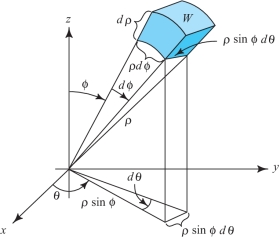
We next use Gauss’ theorem to derive the formula \begin{equation*} \hbox{div }{\bf F}=\frac{1}{\rho^2}\frac{\partial\!}{\partial\! \rho} (\rho^2F_\rho)+\frac{1}{\rho \sin \phi}\frac{\partial\!}{\partial \phi} (\sin \phi \,F_\phi)+\frac{1}{\rho\,\sin \phi} \frac{\partial\! F_\theta}{\partial \theta}\tag{8} \end{equation*} for the divergence of a vector field \({\bf F}\) in spherical coordinates, which was stated in Section 18.2. (Again, the subscripts here denote components, not partial derivatives.) The method is to use the formula \begin{equation*} \hbox{div }{\bf F}({\rm P})=\mathop{\rm limit}_{W\to P}\frac{1}{V(W)} \intop\!\!\!\intop\nolimits_{\partial\! W}{\bf F}\,{\cdot}\,{\bf n}{\,d} S,\tag{9} \end{equation*} where \(W\) is a region with volume \(V(W)\), which shrinks down to a point \({\bf P}\) (in the main text we use a ball, but we can use regions of any shape). Let \(W\) be the shaded region in Figure 18.37.
471
For the two faces orthogonal to the radial direction, the surface integral in equation (9) is, approximately, \begin{equation*} F_\rho(\rho+d\rho,\phi,\theta)\times \hbox{ (area of outer face)}-F_\rho(\rho,\phi,\theta)\times \hbox{ (area of inner face)}\\ \quad \approx F_\rho(\rho+d\rho,\phi,\theta) (\rho+d\rho)^2\sin\phi {\,d}\phi {\,d}\theta - F_\rho(\rho,\phi,\theta)\rho^2\sin \phi {\,d}\phi {\,d}\theta\\[2pt] \quad\approx \frac{\partial\!}{\partial\! \rho} (F_\rho\rho^2 \sin \phi){\,d}\rho {\,d}\phi {\,d}\theta\tag{10} \end{equation*} by the one-variable mean-value theorem. Dividing by the volume of the region \(W\), namely, \(\rho^2\sin\phi {\,d}\rho {\,d}\phi {\,d}\theta\), we see that the contribution to the right-hand side of equation (9) is \begin{equation*} \frac{1}{\rho^2}\frac{\partial\!}{\partial\! \rho}(\rho^2F_\rho)\tag{11} \end{equation*} for these faces. Likewise, the contribution from the faces orthogonal to the \(\phi\) direction is \[ \frac{1}{\rho\sin\phi} \frac{\partial\!}{\partial \phi} (\sin\phi F_\phi), \qquad\hbox{and for the \(\theta\) direction},\qquad \frac{1}{\rho\sin\phi} \frac{\partial\! F_\theta}{\partial \theta}. \]
Substituting (11) and these expressions in equation (9) and taking the limit gives equation (8).
Maxwell’s Equations and the Prediction of Radio Waves: The Communication Revolution Begins
We now discuss Maxwell’s equations, which govern the propagation of electromagnetic fields. The form of these equations depends on the physical units one is employing, and changing units introduces factors like \(4\pi\) and the velocity of light. We shall choose the system in which Maxwell’s equations are simplest.
472
Let \({\bf E}\) and \({\bf H}\) be \(C^{1}\) functions of (\(t\hbox{, } x\hbox{, } y\hbox{, } z\)) that are vector fields for each \(t\). They satisfy (by definition) Maxwell’s equation with charge density \(\rho (t\hbox{, } x\hbox{, } y\hbox{, } z\)) and current density \({\bf J}(t\hbox{, } x\hbox{, } y\hbox{, } z)\) when the following conditions hold: \begin{equation*} \nabla \, {\cdot}\, {\bf E} = \rho \hbox{ (Gauss’ law), }\tag{12} \end{equation*} \begin{equation*} \nabla \, {\cdot}\, {\bf H} = 0 \hbox{ (no negative sources), }\tag{13} \end{equation*} \begin{equation*} \nabla \times {\bf E} + \frac{\partial {\bf H}}{\partial t} = {0} \hbox{ (Faraday’s law), }\tag{14} \end{equation*} and \begin{equation*} \nabla \times {\bf H}- \frac{\partial {\bf E}}{\partial t} = J \hbox{ (Ampère’s law). }\tag{15} \end{equation*}
Of these laws, equations (4) and (6) were described in integral form in Section 18.2 and Section 18.4; historically, they arose in these forms as physically observed laws. Ampère’s law was mentioned for a special case in Section 7.2, Example 12.
Physically, we interpret \({\bf E}\) as the electric field and \({\bf H}\) as the magnetic field. According to the preceding equations, as time \(t\) progresses, these fields interact with each other, and with any charges and currents that are present. For example, the propagation of electromagnetic waves (TV signals, radio waves, light from the sun, etc.) in a vacuum is governed by these equations with \({\bf J} = 0\) and \(\rho\) = 0.
Because \(\nabla \, {\cdot}\, {\bf H} = 0\), we can apply Theorem 8 (from Section 18.3) to conclude that \({\bf H} = \nabla \times {\bf A}\) for some vector field \({\bf A}\). (We are assuming that \({\bf H}\) is defined on all of \({\mathbb R}^{3}\) for each time \(t\).) The vector field \({\bf A}\) is not unique, and we can use \({\bf A^\prime } = {\bf A} + \nabla f\) equally well for any function \(f(t\hbox{, } x\hbox{, } y\hbox{, } z)\), because \(\nabla \times \nabla f = 0\). (This freedom in the choice of \({\bf A}\) is called gauge freedom.) For any such choice of \({\bf A}\), we have, by equation (6), \begin{eqnarray*} {0}=\nabla \times {\bf E} + \frac{\partial {\bf H}}{\partial t} &=& \nabla \times {\bf E} + \frac{\partial\!}{\partial t}\nabla \times {\bf A}\\[6pt] &=& \nabla \times {\bf E} \times \nabla \times \frac{\partial {\bf A}}{\partial t}\\[6pt] &=& \nabla \times \left( {\bf E} + \frac{\partial {\bf A}}{\partial t}\right).\\[-12pt] \end{eqnarray*}
Applying Theorem 7 (from Section 18.3), there is a real-valued function \(\phi \) on \({\mathbb{R}}^{3}\) such that \[ {\bf E} + \frac{\partial {\bf A}}{\partial t} = - \nabla \phi. \]
Substituting this equation and \({\bf H} = \nabla \times {\bf A}\) into equation (7), and using the vector identity (whose proof we leave as an exercise) \[ \nabla \times (\nabla \times {\bf A}) = \nabla (\nabla \, {\cdot}\, {\bf A}) -\nabla^2 {\bf A}, \] we get \begin{eqnarray*} {\bf J} & = & \nabla \times {\bf H} - \frac{\partial {\bf E}}{\partial t} = \nabla \times (\nabla \times {\bf A}) -\frac{\partial\! }{\partial t}\left( -\frac{\partial {\bf A}}{\partial t} - \nabla \phi\right) \\ &=& \nabla (\nabla \, {\cdot}\, {\bf A}) -\nabla^2 {\bf A} + \frac{\partial^2 {\bf A}}{\partial t^2} + \frac{\partial\! }{\partial t} (\nabla \phi). \\[-6pt] \end{eqnarray*}
473
Thus, \[ \nabla^2{\bf A} - \frac{\partial^2 {\bf A}}{\partial t^2} = - {\bf J} + \nabla (\nabla \, {\cdot}\, {\bf A}) + \frac{\partial\!}{\partial t} (\nabla \phi). \]
That is, \begin{equation*} \nabla^2{\bf A} - \frac{\partial^2 {\bf A}}{\partial t^2} = - {\bf J} + \nabla \left(\nabla \, {\cdot}\, {\bf A} + \frac{\partial \phi}{\partial t}\right).\tag{16} \end{equation*}
Again using the equation \({\bf E} + \partial {\bf A}/ \partial t = - \nabla \phi\) and the equation \(\nabla \, {\cdot}\, {\bf E} = \rho\), we obtain \[ \rho = \nabla \, {\cdot}\, {\bf E} = \nabla \, {\cdot}\, \left(-\nabla \phi - \frac{\partial {\bf A}}{\partial t}\right) = - \nabla^2 \phi - \frac{\partial (\nabla \, {\cdot}\, {\bf A})}{\partial t}. \]
That is, \begin{equation*} \nabla^2\phi =-\rho - \frac{\partial (\nabla \, {\cdot}\, {\bf A})}{\partial t}.\tag{17} \end{equation*}
Now let us exploit the freedom in our choice of \({\bf A}\). We impose the “condition” \begin{equation*} \nabla \, {\cdot}\, {\bf A} + \frac{\partial \phi}{\partial t} =0.\tag{18} \end{equation*}
We must be sure we can do this. Supposing we have a given \({\bf A}_{0}\) and a corresponding \(\phi _{0}\), can we choose a new \({\bf A} = {\bf A}_{0} + \nabla\!f\) and then a new \(\phi\) such that \(\nabla \, {\cdot}\, {\bf A} + \partial \phi / \partial t = 0\)? With this new \({\bf A}\), the new \(\phi\) is \(\phi _{0} - \partial\! f/\partial t\); we leave verification as an exercise for the reader. Condition (10) on \(f\) then becomes \[ 0=\nabla\, {\cdot}\, ({\bf A}_{0} + \nabla\!f) = \frac{\partial (\phi_0-\partial\! f/\partial t)}{\partial t} = \nabla \, {\cdot}\, {\bf A}_0 + \nabla^2 f + \frac{\partial \phi_0}{\partial t} -\frac{\partial^2 f}{\partial t^2} \] or \begin{equation*} \nabla^2 f - \frac{\partial^2 f}{\partial t^2} = -\left(\nabla \, {\cdot}\, {\bf A}_0 + \frac{\partial \phi_0}{\partial t}\right).\tag{19} \end{equation*}
Thus, to be able to choose \({\bf A}\) and \(\phi\) satisfying \(\nabla \, {\cdot} \, {\bf A} + \partial \phi /\partial t = 0\), we must be able to solve equation (11) for \(f\). We can indeed do this under general conditions, although we do not prove it here. Equation (11) is called the inhomogeneous wave equation.
If we accept that \({\bf A}\) and \(\phi\) can be chosen to satisfy \(\nabla \, {\cdot} \, {\bf A} + \partial \phi /\partial t = 0\), then equations (8) and (9) for \({\bf A}\) and \(\phi\) become \begin{equation*} \nabla^2{\bf A} -\frac{\partial^2{\bf A}}{\partial t^2} = -{\bf J};\tag{8'} \end{equation*} \begin{equation*} \nabla^2\phi -\frac{\partial^2 \phi}{\partial t^2} = - \rho.\tag{9'} \end{equation*}
Conversely, if \({\bf A}\) and \(\phi\) satisfy the equations \(\nabla \, {\cdot} \, {\bf A} + \partial \phi /\partial t = 0, \nabla ^{2}\phi - \partial ^{2}\phi /\partial t^{2} = - \rho\), and \(\nabla ^{2} {\bf A} - \partial ^{2} {\bf A}/\partial t^{2} = -{\bf J}\), then \({\bf E} = - \nabla \phi - \partial {\bf A}/\partial t\) and \({\bf H} = \nabla \times {\bf A}\) satisfy Maxwell’s equations. This procedure then “reduces” Maxwell’s equations to a study of the wave equation.footnote #
474
Since the eighteenth century, solutions to the wave equation have been well studied (one learns these in most courses on differential equations). To indicate the wavelike nature of the solutions, for example, observe that for any function \(f\), \[ \phi (t,x,y,z) =f(x-t) \] solves the wave equation \(\nabla ^{2}\phi - (\partial ^{2}\phi /\partial t^{2}) = 0\). This solution just propagates the graph of \(f\) like a wave; thus, we might conjecture that solutions of Maxwell’s equations are wavelike in nature. Historically, all of this was Maxwell’s great achievement, and it soon led to Hertz’s discovery of radio waves.
Mathematics again shows its uncanny ability not only to describe but to predict natural phenomena.
For an interesting application of this theory to solving certain differential equations of Mechanics and Technology, including the derivation of Euler's equation of a perfect fluid, click here.
Isaac Newton reputedly said, ''All in nature reduces to differential equations.'' This point of view was paraphrased by Max Planck (see the Historical Note in Section 13.3): ''\(\ldots\) Present day physics, as far as it is theoretically organized, is completely governed by a system of space--time differential equations.''
In this section, we apply the central theorems of vector analysis to the derivation of the differential equations governing heat transfer, electromagnetism, and the motion of some fluids. Keep in mind the importance of these problems in modern technology. For example, a good understanding of fluids and the ability to do computations to solve their governing equations is at the heart of how one builds a modern airplane or designs a submarine. For instance, the flow of air (the fluid in this case) over the wings of an aircraft is very subtle, even though the governing equations are relatively simple. We shall derive a slightly idealized form of these equations in this section. Likewise, the equations of electromagnetism, as we will discuss in the following paragraphs, is central to the communications industry; wireless, television, and much of the operation of modern electronic devices, including computers, depends on these and related fundamental equations.
Conservation Laws
As preparation for deriving the equations of a fluid, let us first discuss an important equation that is referred to as a conservation equation. For fluids, it expresses the conservation of mass; for electromagnetic theory, it expresses the conservation of charge. We shall apply these ideas to the equation for heat conduction and to electromagnetism.
Let \({\bf V}(t, x, y, z)\) be a \(C^{1}\) vector field on \({\mathbb{R}}^{3}\) for each \(t\) and let \(\rho (t, x, y, z)\) be a \(C^{1}\) real-valued function. By the law of conservation of mass for {\bf V} and \(\rho \), we mean that the condition \[ \frac{d}{dt}\iiint\nolimits_W \rho dV = -\iint\nolimits_{\partial W} {\bf J}\, {\bf \cdot}\, {\bf n}\, dS \] holds for all regions \(W\) in \({\mathbb R}^{3}\), where \({\bf J} = \rho {\bf V}\) (see Figure 18.38).
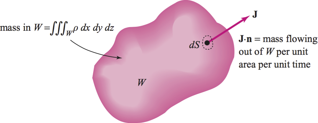
If we think of \(\rho \) as a mass density (\(\rho \) could also be a charge density)---that is, the mass per unit volume---and of \({\bf V}\) as the velocity field of a fluid, the condition simply says that the rate of change of total mass in \(W\) equals the rate at which mass flows \({\it into} \ W\) Recall that \(\iint_{\partial W} {\bf J}\, {\bf \cdot}\, {\bf n}\, dS\) is called the flux of \({\bf J}\). We need the following result.
\(\bf Theorem \quad\) For \({\bf V}\) and \(\rho \) (a smooth vector field and a scalar field on \({\mathbb{R}}^{3})\), the law of conservation of mass for \({\bf V}\) and \(\rho \) is equivalent to the condition \begin{equation} \label {8.5suppl eq1} \hbox{div}\ {\bf J} + \frac{\partial \rho}{\partial t} = 0. \tag{1} \end{equation} That is, \begin{equation} \label {8.5suppl eq2} \rho \hbox{ div } {\bf V} + {\bf V}\, {\bf \cdot}\, {\nabla}\rho + \frac{\partial \rho}{\partial t} =0.\tag{2} \end{equation} Here, div \({\bf J}\) means that we compute div \({\bf J}\) for \(t\) held fixed, and \(\partial \rho /\partial t\) means we differentiate \(\rho \) with respect to \(t\) for \(x, y, z\) fixed.
\(\bf proof\)
First, observe that by differentiating under the integral, we get \[ \frac{d}{dt} \iiint\nolimits_W \rho\ dx dy dz = \iiint\nolimits_W \frac{\partial \rho}{\partial t} \ dx dy dz \] and also \[ \iint\nolimits_{\partial W} {\bf J} \, {\bf \cdot}\, {\bf n}\ dS = \iiint\nolimits_W \hbox{ div } {\bf J}\ d\kern1pt{\bf V} \] by the divergence theorem. Thus, conservation of mass is equivalent to the condition \[ \iiint\nolimits_{W} \left(\hbox{div}\ {\bf J} + \frac{\partial \rho}{\partial t} \right)\!\! \ dx dy dz =0. \] Because this is to hold for all regions \(W\), it is equivalent to div \({\bf J} + \partial \rho / \partial t = 0\). \(\blacklozenge\)
The equation div \({\bf J} + \partial \rho / \partial t = 0\) is called the equation of continuity. An interesting remark is that using the change of variables formula, the law of conservation of mass may be shown to be equivalent to the condition \[ \frac{d}{dt} \iiint\nolimits_{W_t} \rho \ dV = 0, \] where \(W_{t}\) is the image of \(W\) obtained by moving each point in \(W\) along flow lines of \({\bf V}\) for time \(t.\) This result is a special case of the transport theorem that we discuss next.
The Transport Theorem
The transport theorem is an interesting application of the divergence theorem that will be needed in our derivation of the equations of a fluid.
\(\bf Theorem \quad\) Let \({\bf F}\) be a vector field on \({\mathbb{R}}^{3}\) and denote the flow line of \({\bf F}\) starting at \({\bf x}\) after time \(t\) by \(\phi ({\bf x}, t)\). Let \(J({\bf x}, t)\) be the Jacobian of the map \(\phi _{t}\kern-3pt: {\bf x} \mapsto \phi ({\bf x}, t)\) for \(t\) fixed. Then \[ \frac{\partial}{\partial t} J({\bf x}, t) = [\hbox{div } {\bf F}(\phi({\bf x}, t))] \ J ({\bf x},t). \] For a given function \(f(x, y, z, t)\) and a region \(W \subset {\mathbb{ R}}^{3}\), the transport equation holds: \[ \frac{d}{dt}\iiint\nolimits_{W_t} f(x,y,z, t) \ dx dy dz = \iiint\nolimits_{W_t}\left(\frac{Df}{Dt}+ f \hbox{ div }{\bf F} \right) \!\! \ dx dy dz, \] where \(W_{t}=\phi _{t}(W\kern1pt)\), which is the region moving with the flow, and where \[ \frac{Df}{Dt} = \partial f /\partial t + \nabla f\, {\bf \cdot}\, {\bf F} \] is the material derivative.
Taking \(f = 1\), the theorem above implies that the following assertions are equivalent (which justifies the use of the term incompressible):
\(\quad\) 1. \(\hbox{ div } {\bf F} = 0\)
\(\quad\)2. \(\hbox{ volume }(W_{t}) = \hbox{volume }(W\kern.5pt)\)
\(\quad\)3. \(J({\bf x}, t) = 1\)
Let \(\phi \), \(J,\) \({\bf F}\), \(f\) be as just defined. There is also a vector form of the transport theorem, namely, \begin{eqnarray*} \frac{d}{dt} \iiint\nolimits_{W_t}\ (f{\bf F}) \ dx dy dz\hskip15pc\\ =\iiint\nolimits_{W_t} \left[\frac{\partial}{\partial t}(f\kern1pt {\bf F}) + {\bf F} \, {\bf \cdot}\, \nabla (f\kern1pt {\bf F}) + (f\kern1pt {\bf F}) \hbox{ div } {\bf F} \right] \!\! \ dx dy dz, \end{eqnarray*} where \({\bf F} \, {\bf \cdot}\, \nabla (f\kern1pt {\bf F})\) denotes the \(3 \times 3\) derivative matrix \({\bf D} (f\kern1pt {\bf F})\) operating on the column vector \({\bf F}\); in Cartesian coordinates, \({\bf F} \, {\bf \cdot}\, \nabla {\bf G}\) is the vector whose \(i\)th component is \[ \sum^3_{j=1} F_{j} \frac{\partial G^i}{\partial x_j} = F_1\frac{\partial G^i}{\partial x} +F_{2} \frac{\partial G^i}{\partial y} + F_3\frac{\partial G^i}{\partial z}. \] We shall leave the proofs of these results, which are extensions of the arguments used to prove the first theorem above, to the reader.
Derivation of Euler's Equation of a Perfect Fluid
The continuity equation is not sufficient to completely determine the motion of a fluid---we need other conditions.
The fluids that the continuity equation governs can be compressible. If div \({\bf V} = 0\) (incompressible case) and \(\rho \) is constant, equation (\ref{8.5suppl eq2}) follows automatically. But in general, even for incompressible fluids, the equation is not automatic, because \(\rho \) can depend on (\(x, y, z)\) and \(t.\) Thus, even if the equation div \({\bf V} = 0\) holds, div (\(\rho {\bf V}) \ne \) 0 may still be true.
Here we discuss Euler's equation for a perfect fluid. Consider a nonviscous fluid moving in space with a velocity field \({\bf V}\). When we say that the fluid is perfect, we mean that if \(W\) is any portion of the fluid, forces of pressure act on the boundary of \(W\) along its normal. We assume that the force per unit area acting on \(\partial W\) is --\(p\){\bf n}, where \(p\)({\it x, y, z, t}) is some function called the pressure (see Figure 18.39). Thus, the total pressure force acting on \(W\) is \[ {\bf F}_{\partial W} = \hbox{ force } = - \iint\nolimits_{\partial W} p{\bf n}\ {\it dS}. \]
This is a vector quantity; the \(i\)th component of \({\bf F}_{\partial W}\) is the integral of the \(i\)th component of \(p{\bf n }\) over the surface \(\partial W\) (this is therefore the surface integral of a real-valued function). If \({\bf e}\) is any fixed vector in space, we have \[ {\bf F}_{\partial W} \, {\bf \cdot}\, {\bf e} = -\iint\nolimits_{\partial W} p{\bf e} \, {\bf \cdot}\, {\bf n}\, dS,\] which is the integral of a scalar over \(\partial W.\) By the divergence theorem and identity (7) in the table of vector identities (Section 14.7), we get \[ {\bf E} \, {\bf \cdot}\, {\bf F}_{\partial W} = - \iiint\nolimits_{W} \hbox{ div } (\kern1ptp{\bf E}) \ dx dy dz = - \iiint\nolimits_{W} \hbox{ (grad} \ {\it p}) \, {\bf \cdot}\, {\bf E} \ dx dy dz, \] so that \[ {\bf F}_{\partial W} = - \iiint\nolimits_{W} \nabla p \ dx dy dz. \]

Now we apply Newton's second law to a moving region \(W_{t}.\) As in the transport theorem, \(W_{t} = \phi _{t}(W)\), where \(\phi _{t} ({\bf x}) = \phi ({\bf x}, t)\) denotes the flow of \({\bf V}\). The rate of change of momentum of the fluid in \(W_{t}\) equals the force acting on it: \[ \frac{d}{dt}\iiint\nolimits_{W_t} p{\bf V} \ dx dy dz = {\bf F}_{\partial {W_t}} = \iiint\nolimits_{W_t} \nabla p\ \ dx dy dz . \] We apply the vector form of the transport theorem to the left-hand side to get \[ \iiint\nolimits_{W_t} \left[\frac{\partial}{\partial t}(\rho {\bf V}\kern1pt) + {\bf V} \, {\bf \cdot}\, \nabla (\rho {\bf V}\kern1pt) + p {\bf V} \hbox{ div } {\bf V} \right]\!\! \ dx dy dz = - \iiint\nolimits_{W_t} \nabla p \ dx dy dz . \] Because \(W_{t}\) is arbitrary, this is equivalent to \[ \frac{\partial}{\partial t}(\rho {\bf V}\kern1pt) + {\bf V} \, {\bf \cdot}\, \nabla (\rho {\bf V}\kern1pt) + \rho {\bf V} \hbox{ div }{\bf V} = -\nabla p. \] Simplification using the equation of continuity, namely, formula (\ref{8.5suppl eq2}), gives \begin{equation} \label {8.5suppl eq3} \rho \left(\frac{\partial {\bf V}}{\partial t} + {\bf V} \, {\bf \cdot}\, \nabla {\bf V}\right) =-\nabla p. \tag{3} \end{equation} This is Euler's equation for a perfect fluid. For compressible fluids, \(p\) is a given function of \(\rho \) (for instance, for many gases, \(p = A\rho ^{\gamma }\) for constants \(A\) and \(\gamma )\). On the other hand, if the fluid is incompressible, \(\rho \) is to be determined from the condition div \({\bf V} = 0\). Equations (\ref{8.5suppl eq1}) and (\ref{8.5suppl eq3}) then govern the motion of the fluid.
The equations describing the motion of a fluid were first derived by Leonhard Euler in 1755, in a paper entitled ''General Principles of the Motion of Fluids.''Euler did basic work in mechanics as well as voluminous work in pure mathematics, a small part of which has already been discussed in this book; he essentially began the subject of analytical mechanics (as opposed to the Euclidean geometric methods used by Newton). He is responsible for the equations of a rigid body (equations that apply, for example, to a tumbling satellite) and the formulation of many basic equations of mechanics in terms of variational principles; that is, by the methods of maxima and minima of real-valued functions. Euler wrote the first comprehensive textbook on calculus and contributed to virtually all branches of mathematics. He wrote several books and hundreds of research papers even after he became totally blind, and he was working on a new treatise on fluid mechanics at the time of his death in 1783. Euler's equations for a fluid were eventually modified by Navier and Stokes to include viscous effects; the resulting Navier--Stokes equations are described in virtually every textbook on fluid mechanics (The Clay Foundation has offered a prize of $1 million to anyone who shows that for the incompressible Navier–Stokes equations, smooth data at \(t = 0\) lead to smooth solutions for all \(t > 0\).) Stokes is, of course, also responsible for developing Stokes' theorem, one of the main results discussed in this text!