The Carbon Cycle

In the past 200 years, atmospheric CO₂ concentrations have risen by nearly 50 percent, from about 270 ppm to over 400 ppm (reached in mid-2013). Earth’s atmosphere has not contained this much CO₂ for at least the last 400,000 years, and probably for the last 20 million years. Atmospheric CO₂ concentrations are now increasing at an unprecedented rate of 0.5 percent per year, faster than at any time in recent geologic history.

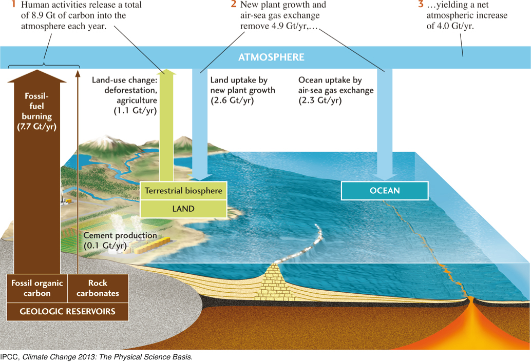
Yet the situation could be worse. Over the decade 2000–2009, human activities injected an average of 8.9 gigatons (Gt) of carbon into the atmosphere each year. (A gigaton, or 1 billion tons, is 10¹² kg, the mass of 1 km³ of water. Note that emissions are calculated in gigatons of carbon, not carbon dioxide. See Exercise 4 at the end of this chapter.) Fossil-fuel burning and other industrial activities emitted about 7.8 Gt/yr of carbon, and the burning of forests and other changes in land use emitted an additional 1.1 Gt/yr. If all of that carbon had stayed in the air, the atmospheric CO₂ increase would have been over 1 percent per year, more than twice the observed rate. Instead, 4.9 Gt of carbon was removed from the atmosphere each year by natural processes. Where did all that carbon go?

We will address this question by examining the carbon cycle: the continual movement of carbon between different components of the Earth system. We touched on the carbon cycle when we discussed biogeochemical cycles—geochemical cycles that involve the biosphere—in Chapter 11. Let’s begin with a broader look at geochemical cycles.

Geochemical Cycles and How They Work

Geochemical cycles are patterns of flow, or flux, of chemicals from one component of the Earth system to another. In discussing geochemical cycles, we view components of the Earth system—atmosphere, hydrosphere, cryosphere, lithosphere, and biosphere—as geochemical reservoirs for the storage of carbon and other chemicals, linked by processes that transport chemicals among them. By quantifying the amounts of the chemicals that are stored in and moved among the various reservoirs, we can gain new insights into the workings of the Earth system.

Residence Time

Reservoirs gain chemicals from inflows and lose chemicals from outflows. If inflow equals outflow, the amount of the chemical in the reservoir stays the same, even though the chemical is constantly entering and leaving it. On average, a molecule of the chemical spends a certain amount of time, called the residence time, in a reservoir.

Think of a crowded bar where many more people want to get in than are allowed by the fire code. After the room fills up, or reaches its capacity, the bouncer begins stopping people at the door. During the busiest hours, when people are waiting to get in, the bar is filled to capacity, or saturated, and is at a steady state, with the number of people going in exactly balancing the number of people coming out. Even though some people come early and stay late and others leave after only a short time, we can calculate an average length of time between arrival and departure—the residence time—by dividing the capacity of the room by the rate of arrivals (inflow) or departures (outflow). If the room’s capacity is 30 people and a new person is let in every 2 minutes on average, the residence time is 60 minutes.

Similarly, we can visualize a chemical’s residence time in the ocean as the average time that elapses between the entry of a molecule of that chemical into the ocean and its removal through sedimentation or some other process. For example, the residence time of sodium in the ocean is extremely long—about 48 million years—because sodium is highly soluble in seawater (that is, the capacity of the reservoir to store sodium is high) and because rivers contain relatively small amounts of sodium (its inflow into the reservoir is low). In contrast, iron has a residence time in the ocean of only about 100 years because its solubility in seawater is very low and the inflow from rivers is relatively high.

Residence times of chemicals in the atmosphere are usually shorter than those in the ocean because the atmosphere is a smaller reservoir than the ocean and fluxes into and out of the atmosphere can be larger. Sulfur dioxide, for example, has a residence time in the atmosphere of hours to weeks, and oxygen, which makes up about 21 percent of the atmosphere, has a residence time of 6000 years. Atmospheric nitrogen gas is abundant (about 78 percent of the atmosphere) and stable and so its residence time is almost 400 million years. A molecule of nitrogen that entered the atmosphere in the late Paleozoic era, about 300 million years ago, is still likely to be there!

Chemical Reactions

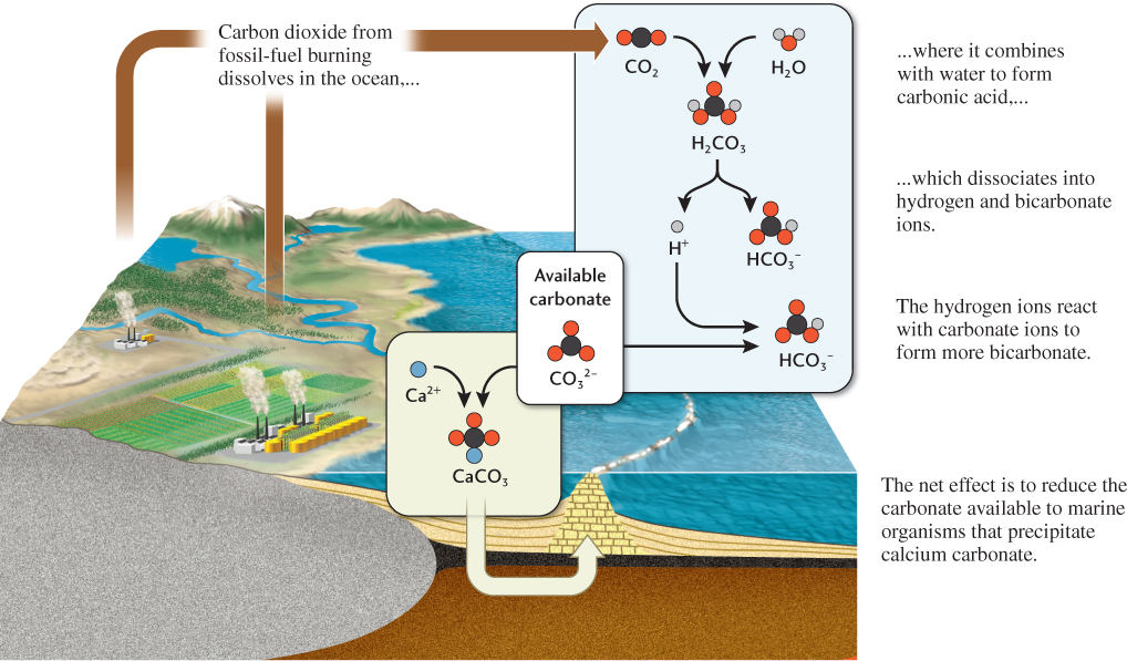
In many cases, reactions with other chemicals govern a chemical’s residence time in a reservoir. For example, as we learned in Chapter 5, a calcium ion (Ca²⁺) can be removed from solution in seawater by reacting with a carbonate ion (CO₃²⁻) to form calcium carbonate (CaCO₃), which can precipitate as carbonate sediment. The amount of calcium that remains dissolved in seawater thus depends on the availability of carbonate ions, which in turn depends on the influx of carbon dioxide (CO₂) into the ocean. When carbon dioxide dissolves in water, most of it reacts with the water to form carbonic acid (H₂CO₃), which can dissociate into hydrogen (H⁺) and bicarbonate ions (HCO₃⁻). Some of the hydrogen ions then react with carbonate ions to form more bicarbonate ions (Figure 15.15). The net effect is to increase the acid content of seawater and decrease the concentration of carbonate ions. The decrease in carbonate affects the ability of marine organisms such as corals, clams, and foraminifera to build their shells and skeletons by precipitating calcium carbonate. As we shall see, this process of ocean acidification is one of the most threatening aspects of anthropogenic global change.

Figure 15.15: Increasing CO₂ concentrations in the atmosphere drive a series of chemical reactions in seawater, causing ocean acidification and reducing the ability of marine organisms to form shells and skeletons of calcium carbonate.

Transport Across Interfaces

Fluxes between reservoirs are governed by processes that transport chemicals into and out of them (Figure 15.16). For example, volcanoes transport gases, aerosols, and dust from the lithosphere into the atmosphere. Wind lifts dust from the lithosphere into the atmosphere, and gravity pulls it back to Earth’s surface. Windborne dust is also an important mechanism for transporting minerals from the lithosphere to the hydrosphere, although by far the largest flux between those two reservoirs comes from minerals dissolved or suspended in rivers.

Figure 15.16: A number of processes result in fluxes of chemicals between components of the climate system.

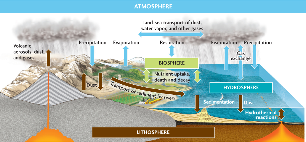
Evaporation and precipitation transport huge amounts of water between the atmosphere and the surfaces of both land and ocean. At the sea surface, gas molecules and salts, in the form of tiny crystals, escape from their dissolved state in the water and enter the atmosphere. That flux is balanced by the dissolution of atmospheric constituents that return to the oceans as rain and by the dissolution of gases directly across the ocean surface.

Sedimentation is the great flux that keeps the ocean in a steady state, primarily by counterbalancing the influx of chemicals in river water. As seafloor sediments are buried, they become part of the oceanic crust. There they stay until they move into the mantle through subduction or become part of the continental crust through accretion. Over the long term, tectonic uplift exposes crustal rocks to weathering and erosion, maintaining the balance of fluxes among the reservoirs.

As we saw in Chapter 11, the biosphere is a unique reservoir because each individual organism interacts constantly with its environment. The most important fluxes into and out of the biosphere are the inflow and outflow of atmospheric gases by respiration, the inflow of nutrients from the lithosphere and hydrosphere, and the outflow of nutrients through the death and decay of organisms. The carbon cycle, which depends critically on the pumping of carbon into and out of the atmosphere by living organisms, is clearly a biogeochemical cycle.

Example: The Calcium Cycle

Before we examine the carbon cycle in more detail, let’s take a look at the calcium cycle, which provides a simpler illustration of the concepts involved in geochemical cycles (Figure 15.17).

Figure 15.17: The calcium cycle, emphasizing fluxes into and out of the ocean. Fluxes are given in gigatons (Gt; 10¹² kg) per year. The inflow of calcium into the ocean approximately balances the outflow.

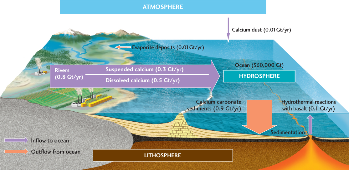
The ocean contains about 560,000 Gt of calcium dissolved in a total ocean mass of about 1.4 × 10⁹ Gt. Calcium steadily enters this reservoir in rivers, which transport large quantities of dissolved and suspended calcium. That calcium is derived from the weathering of carbonate rocks and other minerals such as gypsum and calcium-rich plagioclase feldspar. A much smaller amount of calcium enters the ocean via transport by windblown dust. If the ocean received this continuous inflow of calcium without there being any way to remove it, the ocean would quickly become supersaturated with calcium. The flux that keeps the amount of calcium in the ocean relatively constant is the precipitation of calcium carbonate, as described above. A smaller amount of calcium is precipitated as gypsum in evaporites. Over much longer time scales, calcium-rich sediments are uplifted and weathered, and the calcium they contain is returned to the ocean.

The amount of calcium the ocean can hold is much larger than the inflow and outflow of calcium, so calcium has a fairly long residence time in the ocean. By dividing the total annual influx (0.9 Gt/year) by the ocean’s calcium capacity (560,000 Gt), we obtain a residence time of about 600,000 years.

The Cycling of Carbon

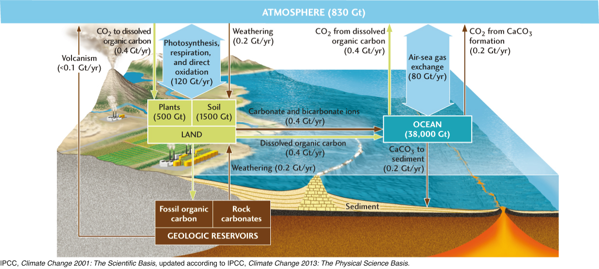
Carbon cycles among four main reservoirs: the atmosphere; the oceans, including marine organisms; the land surface, including plants and soils; and the deeper lithosphere (Figure 15.18). We can describe the flux of carbon among these reservoirs in terms of several basic subcycles. During times when Earth’s climate is stable, each subcycle can be characterized by a constant flux.

Figure 15.18: The carbon cycle describes the fluxes of carbon between the atmosphere and its other principal reservoirs. Amounts of carbon stored in each reservoir are given in gigatons; fluxes are given in gigatons per year.

Atmosphere-Ocean Gas Exchange

The exchange of CO₂ directly across the interface between the oceans and the atmosphere amounts to an average carbon flux of about 80 Gt per year. The flux through this subcycle depends on many factors, including air and sea temperatures and the composition of the seawater, but it is particularly sensitive to wind velocity, which increases the transfer of CO₂ and other gases by stirring up the surface water and generating sea spray. Carbon dioxide dissolved in seawater escapes from solution and enters the atmosphere by evaporating from sea spray, while atmospheric CO₂ enters the ocean by dissolving in sea spray and rain or directly across the sea surface.

Atmosphere-Biosphere Gas Exchange

The subcycle with the greatest carbon flux, 120 Gt per year, is the exchange of CO₂ between the terrestrial biosphere and the atmosphere by photosynthesis, respiration, and decomposition. Plants take in this entire amount of CO₂ during photosynthesis and respire about half of it back into the atmosphere. The other half is incorporated into plant tissues—leaves, wood, and roots—as organic carbon. Animals eat the plants, and microorganisms decompose them; both processes result in the breakdown of plant tissues and the respiration of CO₂. Much of the organic carbon released by these processes—about three times the total plant mass—is stored in soils. A significant fraction (about 4 Gt/year) reenters the atmosphere through direct oxidation by forest fires and other combustion of plant material.

A small fraction of the CO₂ incorporated into plant tissues (0.4 Gt/year) is dissolved in surface waters and transported by rivers to the ocean, where it is respired back into the atmosphere by marine organisms and eventually taken up again by plants through photosynthesis.

Lithosphere-Atmosphere Gas Exchange

The weathering of carbonate rock removes about 0.2 Gt of carbon per year from the lithosphere and an equal amount from the atmosphere. The CO₂ dissolved in rainwater forms carbonic acid, which reacts with carbonates in the rock, releasing carbonate and bicarbonate ions, which are transported by rivers to the ocean. Here, shell-forming marine organisms reverse the weathering reaction, precipitating calcium carbonate and releasing an equal amount of carbon back into the atmosphere as CO₂. This subcycle illustrates one way in which the carbon cycle is linked to the calcium cycle.

Another such linkage is through the weathering of silicate rocks, most of which contain significant amounts of calcium. Silicate weathering releases calcium into surface waters, which flow to the ocean, where the calcium ions combine with carbonate ions to form calcium carbonate, thus removing CO₂ from the atmosphere. The net flux of carbon from silicate weathering is relatively small (less than 0.1 Gt/year), so, like volcanism (which releases minor amounts of CO₂ into the atmosphere), it is usually neglected in short-term climate modeling. Over the long term, however, the effects of silicate weathering can be substantial, because, unlike carbonate weathering, it removes CO₂ from the atmosphere and stores it, semi-permanently, in the lithosphere. For example, the uplifting of the Himalaya and the Tibetan Plateau, which began about 40 million years ago, may have increased weathering rates enough to reduce the concentration of CO₂ in the atmosphere, contributing to the subsequent climate cooling that led to the Pleistocene glaciations (see Earth Issues 22.1).

Human Perturbations of the Carbon Cycle

With this background, let’s return to the fate of anthropogenic carbon emissions. Figure 15.19 shows what happened to the carbon that was added to the atmosphere by human activities in the decade 2000-2009. Out of a total of 8.9 Gt/yr injected into the atmosphere by human activities, only 45 percent (4.0 Gt/year) remained in the atmosphere as CO₂. The rest was absorbed in nearly equal amounts by the oceans (2.3 Gt/year) and the land surface (2.6 Gt/year). Through the carbon cycle, the hydrosphere and lithosphere have clearly been doing their fair share of absorbing our increasing carbon emissions!

Figure 15.19: Much of the CO₂ emitted into the atmosphere by human activities is absorbed by the oceans and by plant growth on land. The remainder stays in the atmosphere, increasing the concentration of CO₂. The fluxes shown in this figure (given in gigatons per year) are for the decade 2000–2009.

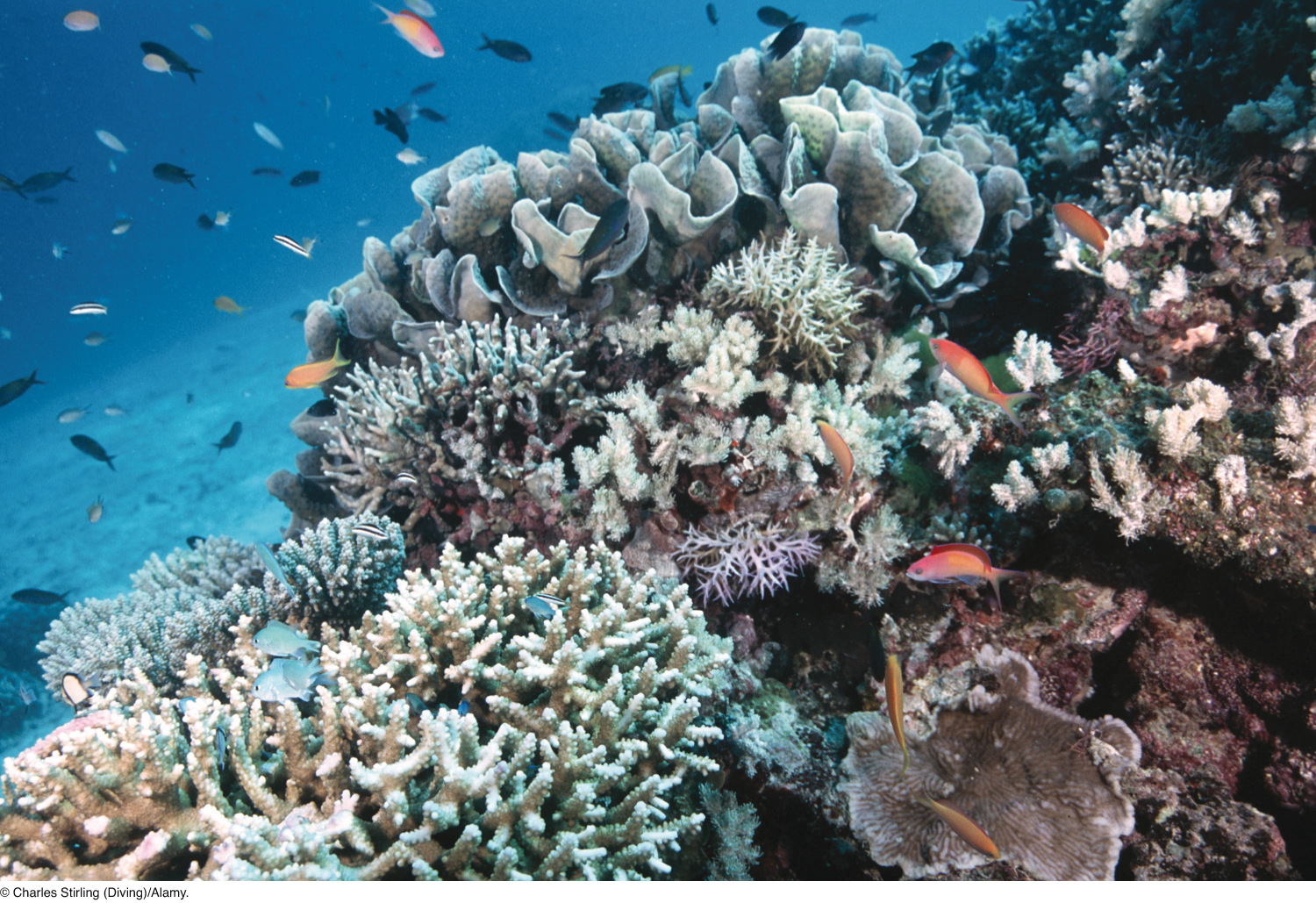
Although this removal of carbon from the atmosphere acts to reduce the rate of global warming—a good thing, no doubt—its effects on marine life can be deadly. Anthropogenic carbon emissions are being absorbed by the oceans, making seawater more acidic, and this ocean acidification is increasing the solubility of calcium in seawater, making it more difficult for key marine organisms to form their calcium carbonate shells and skeletons (see Figure 15.15). Coral reefs are already in trouble (Figure 15.20), and if the present trends continue, ocean acidification could cause population declines in common marine organisms such as starfish and mollusks within the next few decades. In fact, some biologists believe that this type of global change has already contributed to massive die-offs of starfish recently reported on both the east and west coasts of North America.

Figure 15.20: Marine organisms that form their shells or skeletons by precipitating calcium carbonate, such as these corals in the Great Barrier Reef of Australia, are threatened by ocean acidification.

What will happen on land is less clear. In fact, exactly what is happening to the huge amount of carbon dioxide being pulled out of the atmosphere by terrestrial plants has been a real puzzle (see the Practicing Geology exercise at the end of the chapter).