12-3 Spacecraft images show remarkable activity in the clouds of Jupiter and Saturn
Most of our detailed understanding of Jupiter and Saturn comes from a series of robotic spacecraft that have examined these remarkable planets at close range. They found striking evidence of stable, large-scale weather patterns in both planets’ atmospheres, as well as evidence of dynamic changes on smaller scales.
Spacecraft to Jupiter and Saturn
The first several spacecraft to visit Jupiter and Saturn each made a single flyby of the planet. Pioneer 10 flew past Jupiter in December 1973; it was followed a year later by the nearly identical Pioneer 11, which went on to make the first-ever flyby of Saturn in 1979. Also in 1979, another pair of spacecraft, Voyager 1 and Voyager 2, sailed past Jupiter. These spacecraft sent back spectacular close-up color pictures of Jupiter’s dynamic atmosphere. Both Voyagers subsequently flew past Saturn.
The first spacecraft to go into Jupiter orbit was Galileo, which carried out an extensive program of observations from 1995 to 2003. The Cassini spacecraft went into orbit around Saturn in 2004. A cooperative project of NASA, the European Space Agency, and the Italian Space Agency, this spacecraft is named for astronomer Gian Domenico Cassini. On the way to its destination it viewed Jupiter at close range, recording detailed images such as Figure 12-2a. The latest spacecraft, Juno, was launched in 2011, and will reach Jupiter in 2016. By measuring Jupiter’s composition, structure, and magnetic field, Juno should shed light on planet formation, the early solar system, and magnetic dynamos.
Observing Jupiter’s Dynamic Atmosphere
Immense storms on Jupiter and Saturn can last for months or years
While the general pattern of Jupiter’s atmosphere stayed the same during the four years between the Pioneer and Voyager flybys, there were some remarkable changes in the area surrounding the centuries-old Great Red Spot. During the Pioneer flybys, the Great Red Spot was embedded in a broad white zone that dominated the planet’s southern hemisphere (Figure 12-4a). By the time of the Voyager missions, a dark belt had broadened and encroached on the Great Red Spot from the north (Figure 12-4b). In the same way that colliding weather systems in our atmosphere can produce strong winds and turbulent air, the interaction in Jupiter’s atmosphere between the belt and the Great Red Spot embroiled the entire region in turbulence (Figure 12-5). By 1995, the Great Red Spot was once again centered within a white zone (Figure 12-4c); when Cassini flew past Jupiter in 2000, the dark belt to the north of the Great Red Spot embroiled the entire region in turbulence.
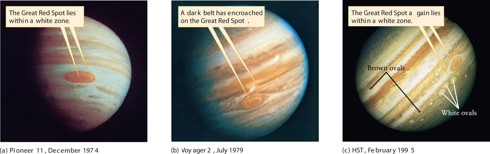
Jupiter’s Changing Appearance These images from (a), (b) spacecraft and (c) the Hubble Space Telescope show major changes in the planet’s upper atmosphere over a 20-year period.
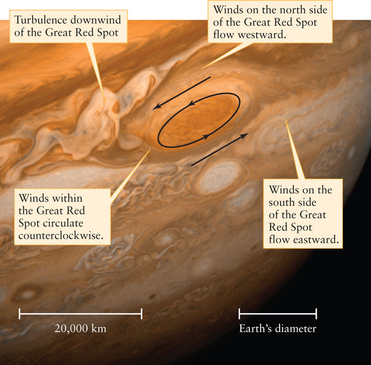
 The Great Red Spot This image of the Great Red Spot shows the counterclockwise circulation of gas in the Great Red Spot that takes about 6 days to make one rotation. The clouds that encounter the spot are forced to pass around it, and when other oval features are near it, the entire system becomes particularly turbulent, like batter in a two-bladed blender.
329
Over the past three centuries, Earth-based observers have reported many long-term variations in the Great Red Spot’s size and color. At its largest, it measured 40,000 by 14,000 km—so large that three Earths could fit side by side across it! At other times (as in 1976 and 1977), the spot almost faded from view. During the Voyager flybys of 1979, the Great Red Spot was comparable in size to Earth (see Figure 12-5).
Clouds at different heights within Jupiter’s atmosphere reflect different wavelengths of infrared light. Using this effect, astronomers used an infrared telescope on board the Galileo spacecraft to help clarify the vertical structure of the Great Red Spot. Most of the Great Red Spot is made of clouds at relatively high altitudes, surrounded by a collar of very low-level clouds about 50 km (30 miles, or 160,000 feet) below the high clouds at the center of the spot. This same kind of structure is seen in high-pressure areas in Earth’s atmosphere, although on a much smaller scale.
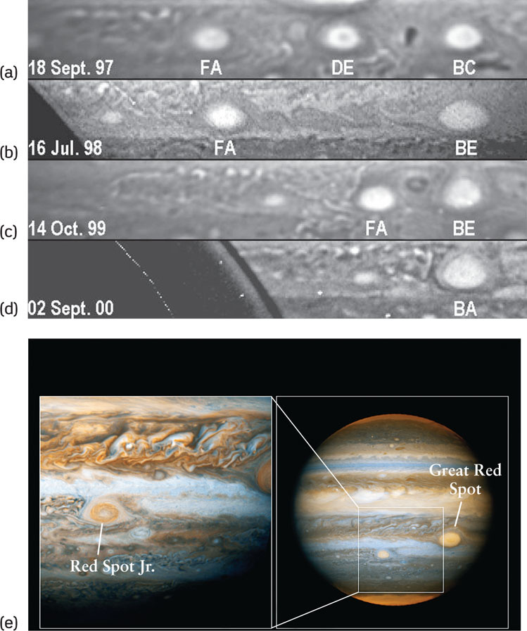
Creating Red Spot Jr. (a–d) For 60 years prior to 1998, the three white ovals labeled FA, DE, and BC traveled together at the same latitude on Jupiter. Between 1998 and 2000, they combined into one white oval, labeled BA, which (e) became a red spot, named Red Spot Jr., in 2006.
Cloud motions in and around the Great Red Spot reveal that the spot rotates counterclockwise and takes about 6 days to complete a full rotation. Furthermore, winds to the north of the spot blow to the west, and winds south of the spot move toward the east. The circulation around the Great Red Spot is thus like a wheel spinning between two oppositely moving surfaces (see Figure 12-5). Weather patterns on Earth tend to change character and eventually dissipate when they move between plains and mountains or between land and sea. But because no solid surface or ocean underlies Jupiter’s clouds, no such changes can occur for the Great Red Spot—which may explain how this wind pattern has survived for at least three centuries.
Other persistent features in Jupiter’s atmosphere are the white ovals. Several white ovals are visible in Figure 12-4c. As in the Great Red Spot, the wind flow in white ovals is counterclockwise. White ovals are also apparently long-lived; Earth-based observers have reported seeing them in the same location since 1938.
Most of the white ovals are observed in Jupiter’s southern hemisphere, whereas brown ovals are more common in Jupiter’s northern hemisphere. Brown ovals appear dark in a visible-light image like Figure 12-4c, but they appear bright in an infrared image. For this reason, brown ovals are understood to be holes in Jupiter’s cloud cover. They permit us to see into the depths of the Jovian atmosphere, where the temperature is higher and the atmosphere emits infrared light more strongly. White ovals, by contrast, have relatively low temperatures. They are areas with cold, high-altitude clouds that block our view of the lower levels of the atmosphere.
330
Between 1998 and 2000 three white ovals merged in Jupiter’s southern hemisphere. The merger of these ovals, each of which had been observed for 60 years, led to the formation of a massive storm about half the size of the Great Red Spot (Figure 12-6). Time will tell whether this new feature—called Red Spot Jr.—is as long-lived as its larger cousin. Even Jupiter’s large belts can disappear. In 2009, Jupiter’s dark southern belt began to fade and was completely gone by June 2010 (Figure 12-7). This disappearing act has occurred about 14 times in the last century.
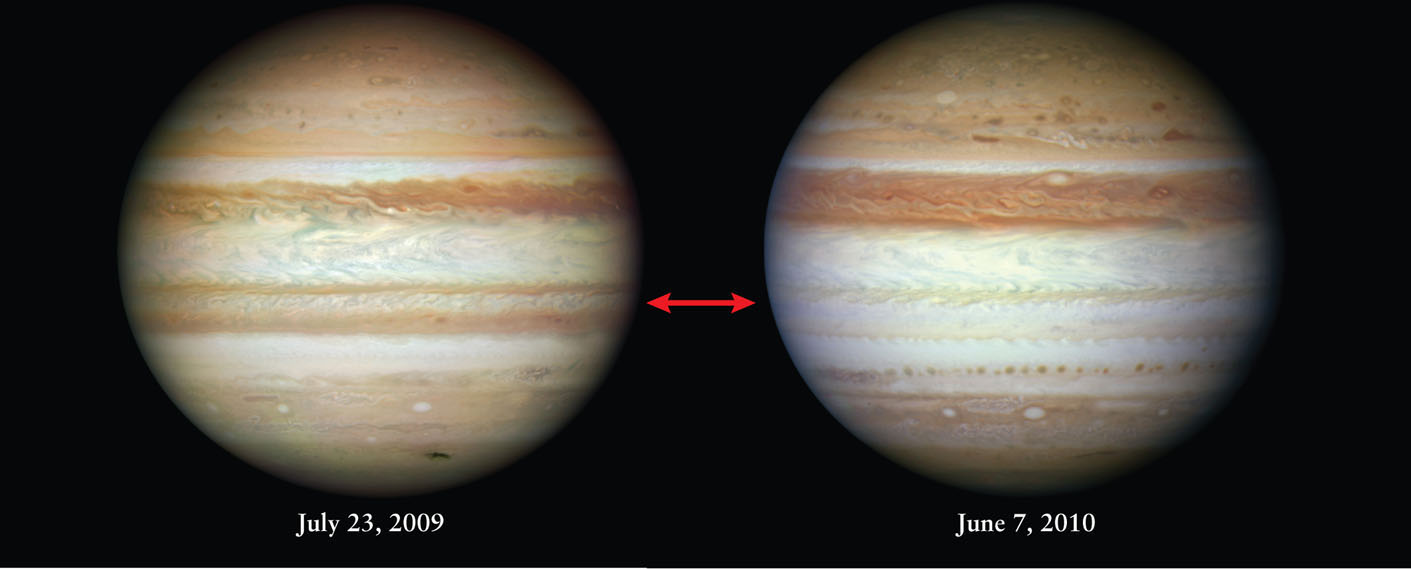
Dark Belt Fades on Jupiter The south equatorial belt completely faded from view between mid-2009 and mid-2010. White-colored ammonia ice crystals appeared at higher elevations, blocking the darker belt from view, but the full mechanism is not understood. By late 2010, the belt began to reappear.
331
CONCEPT CHECK 12-3
Besides color, what are some differences between Jupiter’s white ovals and brown ovals?
Storms and Patterns on Saturn
While Saturn has belts and zones like Jupiter, it has no storm systems as long-lived as Jupiter’s Great Red Spot. But about every 30 years—roughly the orbital period of Saturn—Earth-based observers have reported seeing storms in Saturn’s clouds that last for several days or even months. Figure 12-8 shows one such storm that appeared in Saturn’s southern hemisphere in 2004.
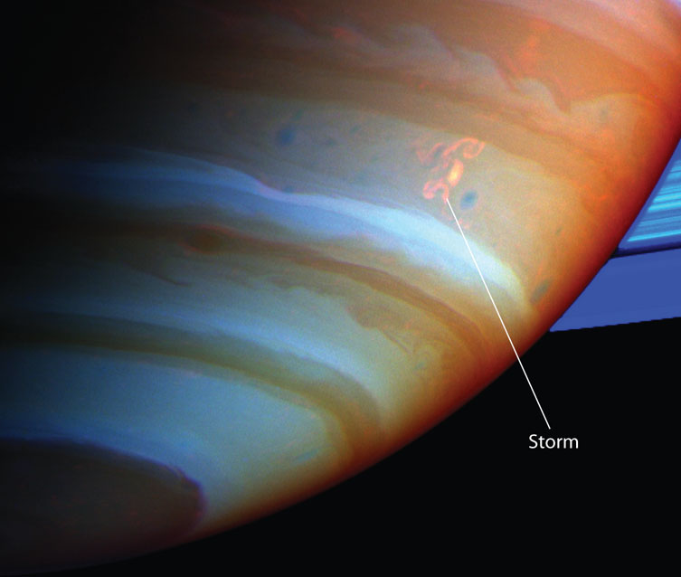
 A New Storm on Saturn This infrared image from the Cassini spacecraft shows a storm the size of Earth that appeared in Saturns southern hemisphere in 2004. Cassini has observed several storms in this same region of Saturn.
 Saturn’s storms are thought to form when warm atmospheric gases rise upward and cool, causing gaseous ammonia to solidify into crystals and form white clouds. On Earth, similar rapid lifting of air occurs within thunderstorms and can cause water droplets to solidify into hailstones. Earth thunderstorms produce electrical discharges (lightning) that generate radio waves, which you hear as “static” on an AM radio. Radio receivers on board Cassini have recorded similar “static” emitted by storms on Saturn, which strongly reinforces the idea that these storms are like thunderstorms on Earth.
Around Saturn’s north pole, an enigmatic hexagonal pattern was glimpsed by Voyager in 1980. Cassini captured this pattern in greater detail, establishing that it persists for more than 26 years (Figure 12-9a). Amazingly, experiments on Earth that simulate Saturn’s atmosphere have recreated this pattern (Figure 12-9b).
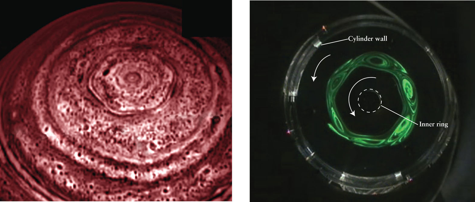
Hexagonal Pattern Around Saturn’s North Pole (a) An infrared image made by Cassini. Each side of the hexagonal pattern is about the diameter of Earth. Inside the hexagon is a rapidly circulating jet stream. (b) Experiments with fluids have recreated the green hexagonal pattern in a cylinder. The cylinder, filled with fluid, spins slowly to simulate Saturn’s overall rotation, while an inner ring is spun faster than the fluid to simulate the jet stream observed around Saturn’s pole. Simulating Saturn’s gaseous atmosphere can be performed with fluids because under the right conditions, fluids and gas behave similarly.
332