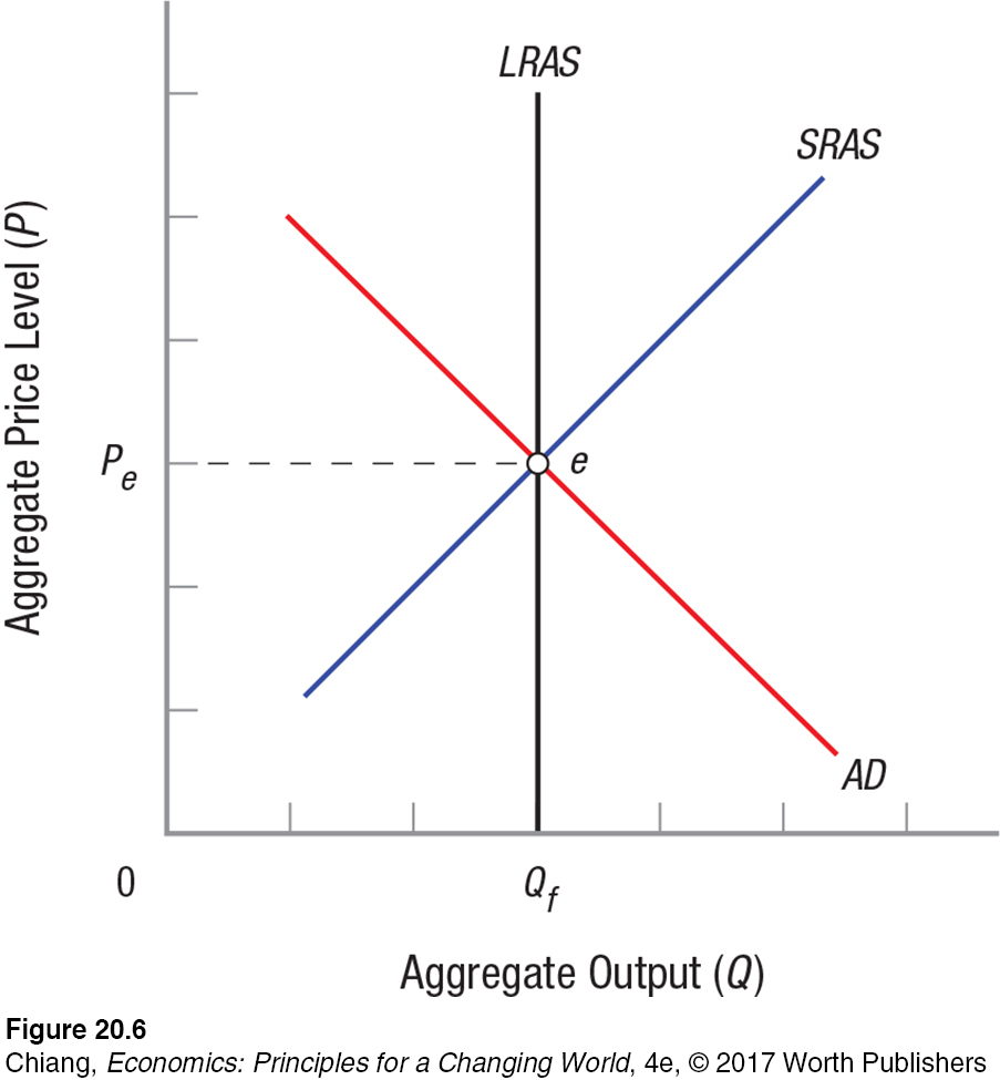
Let us now put together our aggregate demand and aggregate supply model. A short-run macroeconomic equilibrium occurs at the intersection of the short-run aggregate supply and aggregate demand curves; see point e in Figure 6. In this case, point e also represents long-run macroeconomic equilibrium because the economy is operating at full employment, producing output Q_f.

Output level Q_f represents full employment. The SRAS curve assumes price level expectations equal to P_e, and thus Q_f is the natural rate of unemployment or output. Remember that the natural rate of unemployment is that unemployment level at which inflation is low and consistent with inflationary expectations in the economy.

542

The spending multiplier is an important concept introduced into macroeconomics by John Maynard Keynes in 1936. The central idea is that new spending creates more spending, income, and output than just an amount equal to the new spending itself.

Let’s assume, for example, that consumers tend to spend three-quarters and save one-quarter of any new income they receive. Now, assume that good weather encourages a family to spend the day at the annual county fair, spending $100 on food and rides. In other words, $100 of new spending is introduced into the economy. That $100 spent on food and rides adds $100 in income to the operator of the fair, because all spending equals income to someone else (whether that be the owner or the workers she hires). Of this additional income, suppose that $25 is saved and $75 is spent by the fair operator to fix a plumbing leak in her home. That $75 in spending becomes $75 in income to the plumber. Now that the plumber has $75 more income, suppose he saves $18.75 (25% of $75) and uses the rest ($56.25) to change the oil in his car, generating $56.25 in income to the mechanic, and so on, round-by-round.

Adding up all of the new spending (equal to the sum of $100 + $75 + $56.25 + . . . ) from the initial $100 results in total spending increasing by $400. This represents an increase in output or GDP of $400. Adding up total new saving ($25 + 18.75 + . . . ) equals $100, which means that the initial $100 in new spending has increased savings by the same amount through the multiplier process.

The proportion of additional income that consumers spend and save is known as the marginal propensity to consume and the marginal propensity to save (MPC and MPS). In our example, MPC = 0.75 and MPS = 0.25. The multiplier is equal to 4, given that $400 of new income was created with the introduction of $100 of new spending. The formula for the spending multiplier is equal to 1/(1 − MPC) = 1/MPS, and in this case, is 1/(1 − 0.75) = 1/0.25 = 4. This formula works as long as the aggregate price level is stable.

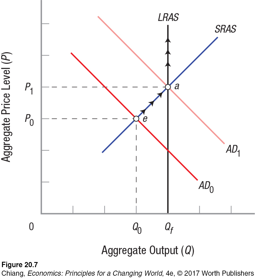
When the economy has many unemployed resources and excess capacity, the price level will remain constant and output will increase by the full magnitude of the multiplier. However, when the economy moves up the SRAS curve in the short run, its response to the same increase in aggregate spending is not as great. In Figure 7, aggregate demand increases the same amount as before. The new equilibrium is at point a with output of Q_f. But, output grows less because price increases or inflation eat up some of each spending round, resulting in less real output. The multiplier is therefore less than the pure spending multiplier of 4 just discussed. Note that once aggregate demand is increased beyond AD₁, price increases soak up the entire increase in aggregate demand (along the LRAS curve) because real output does not change.

543

Let’s take a moment to summarize where we are before we begin to use this model to understand some important macroeconomic events. Short-run macroeconomic equilibrium occurs at the intersection of AD and SRAS. It can also happen that this equilibrium represents long-run equilibrium, but not necessarily; equilibrium can occur at less than full employment. As we will see shortly, the Great Depression is one example of this. Increases in spending are multiplied and lead to greater changes in output than the original change in spending. For policymakers, this means that the difference between equilibrium real GDP and full-employment GDP (the GDP gap) can be closed with a smaller change in spending.

This leads us to the point where we can use the AD/AS model to analyze past macroeconomic events. By looking at these events through the AD/AS lens, we begin to see the options open to policymakers. Let’s now look at what happened during the Great Depression, then examine both demand-pull and cost-push inflation. Each type of inflation presents unique challenges for policymakers.

Figure 6 conveniently showed the economy in long-run equilibrium and short-run equilibrium at the same point. The Great Depression demonstrated, however, that an economy can reach short-run equilibrium at output levels substantially below full employment.

The 1930s Depression was a graphic example of just such a situation. Real GDP dropped by nearly 40% between 1929 and 1933. Unemployment peaked at 25% in 1932 and never fell below 15% throughout the 1930s.

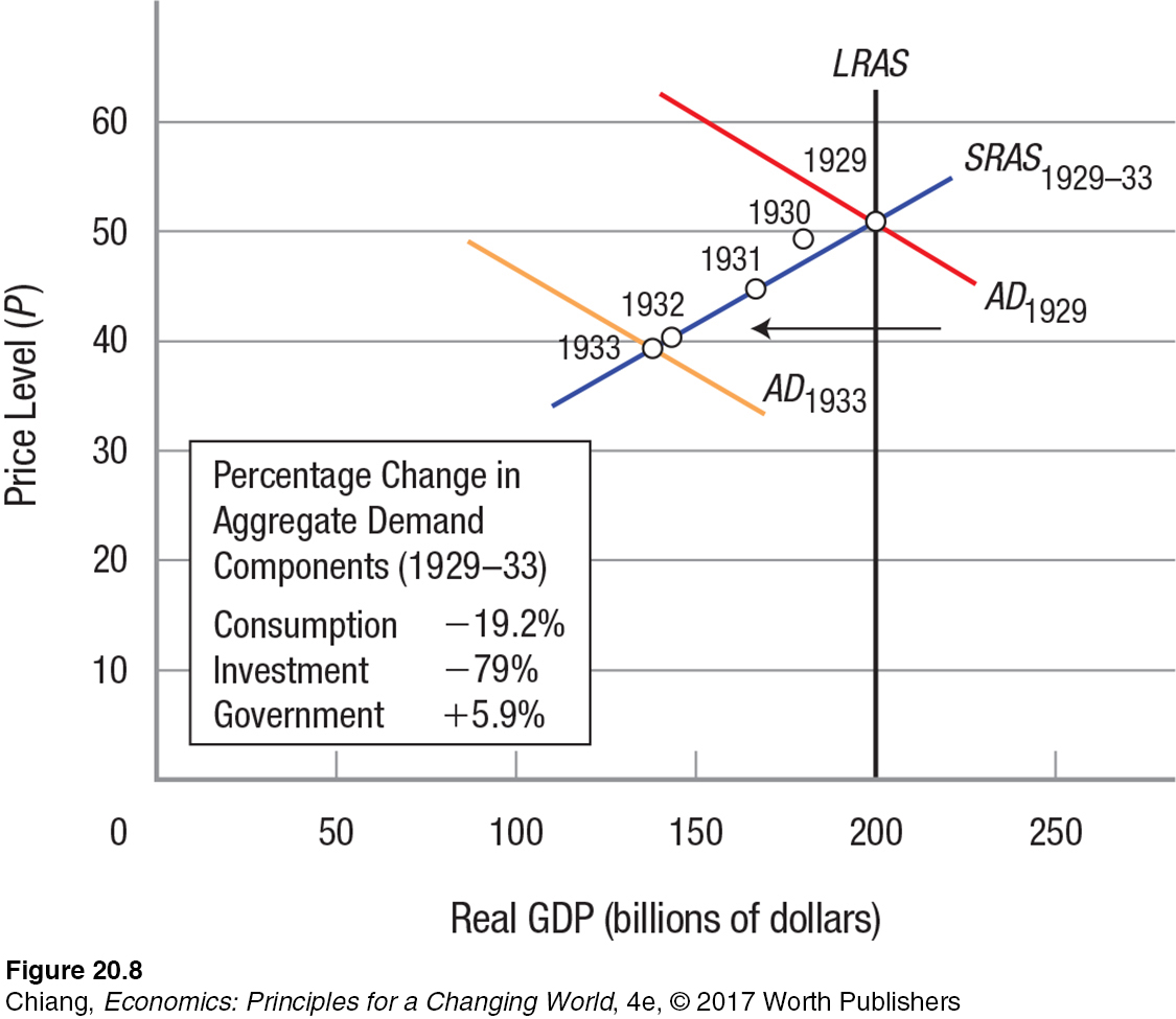
Figure 8 shows the actual data for the Great Depression with superimposed aggregate demand and SRAS curves for 1929 and 1933. Investment is the most volatile of the GDP components, and it fell nearly 80% from 1929 to 1933. This drop in investment reduced spending, and therefore income and consumption, resulting in a deep depression. The increase in aggregate demand necessary to restore the economy back to 1929 levels was huge, and it was no wonder that a 6% increase in government spending had virtually no impact on the Depression. It wasn’t until spending ramped up for World War II that the country moved beyond the Depression.

544

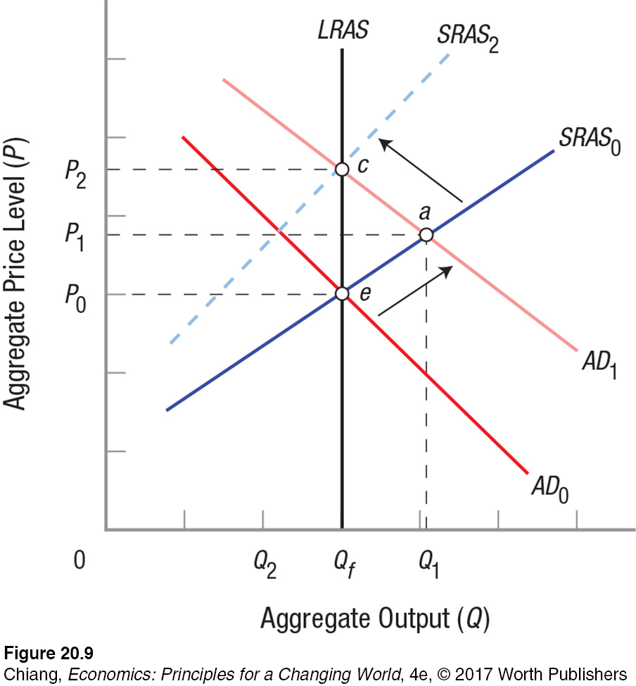
Demand-pull inflation occurs when aggregate demand expands so much that equilibrium output exceeds full employment output. Turning to Figure 9, assume that the economy is initially in long-run equilibrium at point e. If businesses become overly exuberant and expand investments in some area (such as telecommunications in the late 1990s), this expansion will push aggregate demand out to AD₁. The economy moves to a short-run equilibrium beyond full employment (point a), and the price level rises to P₁.

On a temporary basis, the economy can expand beyond full employment as workers incur overtime, temporary workers are added, and more shifts are employed. Yet, these activities increase costs and prices. And because LRAS has not shifted, the economy will ultimately move to point c (if AD stays at AD₁), shifting short-run aggregate supply to SRAS₂ and leaving prices permanently higher (at P₂). In the long run, the economy will gravitate to points such as e and c. Policymakers could return the economy back to the original point e by instituting policies that reduce AD back to AD₀. These might include reduced government spending, higher taxes, or other policies that discourage investment, consumer spending, or exports.

Demand-pull inflation can continue for quite a while, especially if the economy begins on the SRAS curve well below full employment. Inflation often starts out slow and builds up steam.

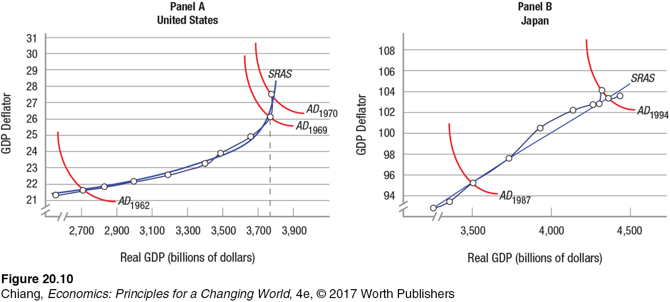
Decade-long demand-pull inflation scenarios for the United States in the 1960s and for Japan in the last half of the 1980s and first half of the 1990s are shown in Figure 10.

For the United States, the slow escalation of the Vietnam conflict fueled a rising economy along the hypothetical short-run aggregate supply curve placed over the data in panel A. Early in the decade, the price level rose slowly as the economy expanded. But notice how the short-run aggregate supply curve began to turn nearly vertical and inflation rates rose as the economy approached full employment in 1969. Real output growth virtually halted between 1969 and 1970, but inflation was 5.3%. The economy had reached its potential.

The Japanese economy during the 1985–1995 period is a different example of demand-pull inflation. Panel B of Figure 10 shows a steadily growing economy with rising prices, throughout the 1980s and early 1990s. Japan ran huge trade surpluses and the yen appreciated (becoming more valuable). A rising yen would eventually reduce exports (Japanese products would become too expensive). To keep this from happening, the Japanese government kept interest rates artificially low, reducing the pressure on the yen and encouraging investment. But these policies fueled a huge real estate and stock bubble that began collapsing in the beginning of the 1990s and led to a decade-long recession that has been called “the lost decade.”

545

Demand-pull inflation can often take a while to become a problem. But once the inflation spiral gains momentum, it can pose a serious problem for policymakers.

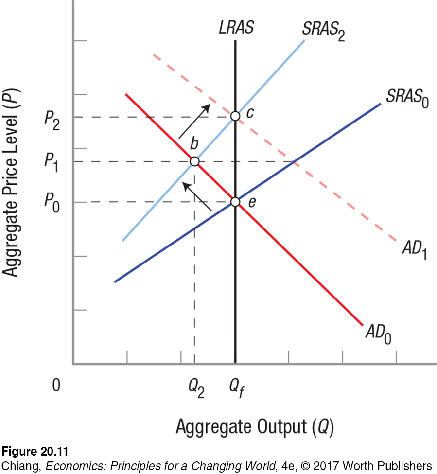
Cost-push inflation occurs when a supply shock hits the economy, shifting the short-run aggregate supply curve leftward, as from SRAS₀ to SRAS₂ in Figure 11. The 1973 oil shock is a classic example. Because oil is a basic input in so many goods and services we purchase, skyrocketing oil prices affected all parts of the economy. After a bout of cost-push inflation, rising resource costs push the economy from point e to point b in Figure 11. Note that at point b, real output has fallen (the economy is in a recession) and the price level has risen. Policymakers can increase demand to AD₁ and move the economy back to full employment at point c. For example, they might increase government spending, reduce taxes, or introduce policies that encourage consumption, investment, or net exports. But notice that this means an even higher price level. Alternatively, policymakers could reduce inflationary pressures by reducing aggregate demand, but this leads to an even deeper recession as output and employment fall further.

546

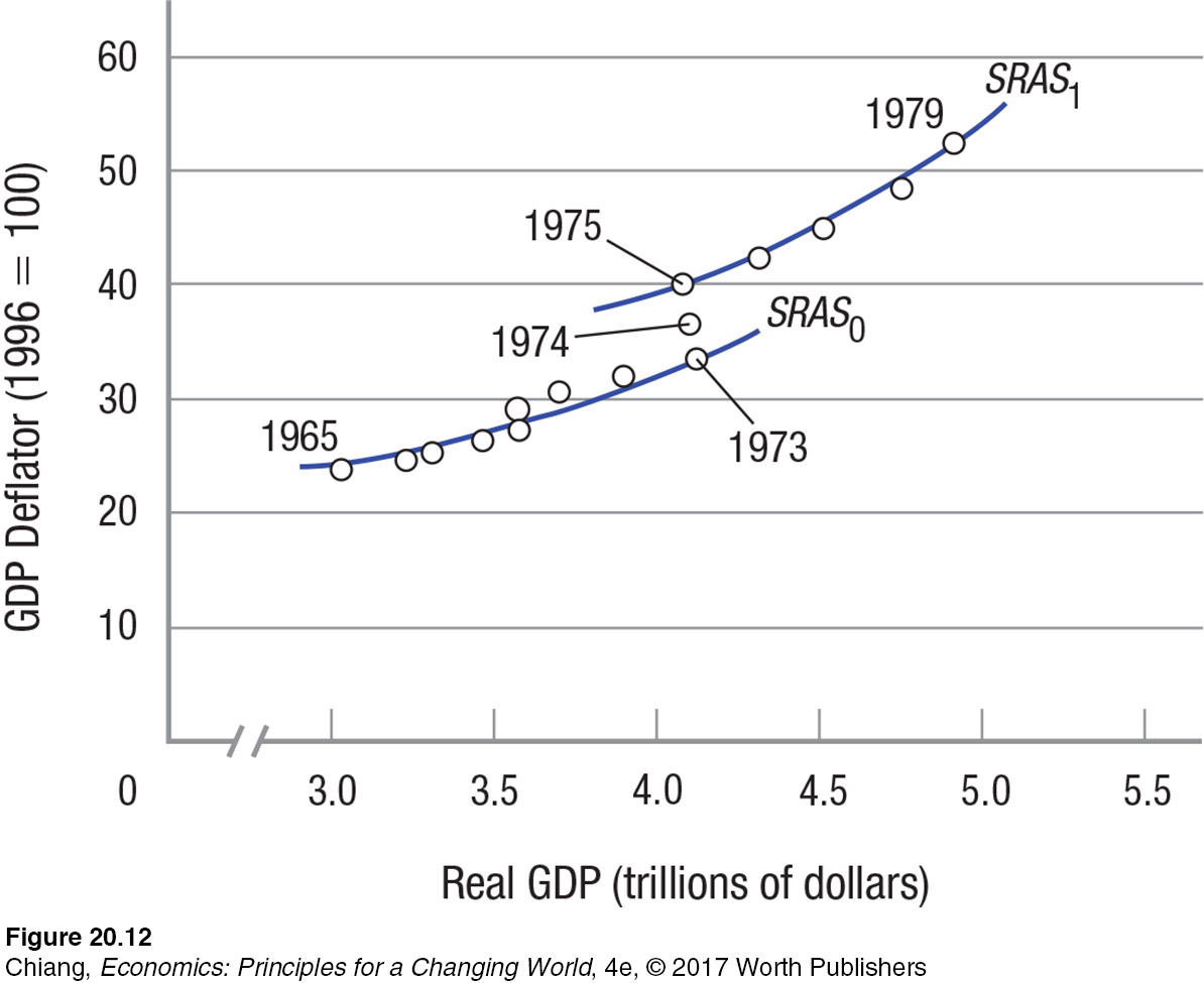
Figure 12 shows the striking leftward shift in equilibrium points for 1973–1975. Output stood still, while prices rose as the economy adjusted to the new energy prices. Superimposed over the annual data are two hypothetical short-run aggregate supply curves. Notice that it took the economy roughly three years to absorb the oil shock. Only after the economy had adjusted to the new prices did it continue on a path roughly equivalent to the pre-1973 SRAS curve.

Before the Great Depression, economic analysis focused on the behavior of individuals, households, and businesses. Little attention was paid to the macroeconomic stabilization potential of government policies. The federal government had its responsibilities under the Constitution in many areas—such as national defense, the enforcement of contracts, and tax collection—but managing the economy was not among them.

The Great Depression of the 1930s and John Maynard Keynes’s The General Theory drastically changed how economists viewed the role of the federal government. During the Depression, when unemployment reached 25% and bank failures wiped out personal savings, federal intervention in the economy became imperative. After the 1930s, the federal government’s role grew to encompass (1) expanded spending and taxation and the resulting exercise of fiscal policy, (2) extensive new regulation of business, and (3) expanded regulation of the banking sector, along with greater exercise of monetary policy.

547

The next chapter focuses on how government spending and taxation combine to expand or contract the macroeconomy. When the economy enters a recession, fiscal policy can be used to moderate the impact and prevent another depression. Later chapters will explore the monetary system and the use of monetary policy to stabilize the economy and the price level. The AD/AS model will serve as a tool to analyze both fiscal and monetary policies. As you read these chapters, keep in mind that the long-run goals of fiscal and monetary policy are economic growth, low unemployment, and modest inflationary pressures.