The persistent unemployment that occurred after the 2007–2009 recession in what is known as a jobless recovery had economists debating the right policy to use. Fiscal policy was undertaken to boost market activity, at the cost of rising debt. And significant monetary policy actions were taken to inject the economy with more money, at the cost of potential inflation. Questions that arise from these policies include whether the effort to reduce unemployment could result in higher inflation, or whether macroeconomic policy has any short-term effects at all. We address these issues in this section by studying two theories developed in the 1950s and 1960s: the Phillips curve and rational expectations.

With Phillips curve analysis, it first seemed that fiscal policy was easy: Pick an unemployment rate from column A and get a corresponding inflation rate from column B. Unfortunately, reality turned out to be much more complex. With rational expectations, the question was whether policy could ever be effective at all.

Does a relationship exist between unemployment and inflation? In his early work, A. W. Phillips compared the rate of change in money wages to unemployment rates in Britain over the years 1861 to 1957. The negatively sloped curve shown in Figure 1 reflects his estimate of how these variables were related and has been called a Phillips curve in his honor. As you can see, when unemployment rises, wage rates fall.

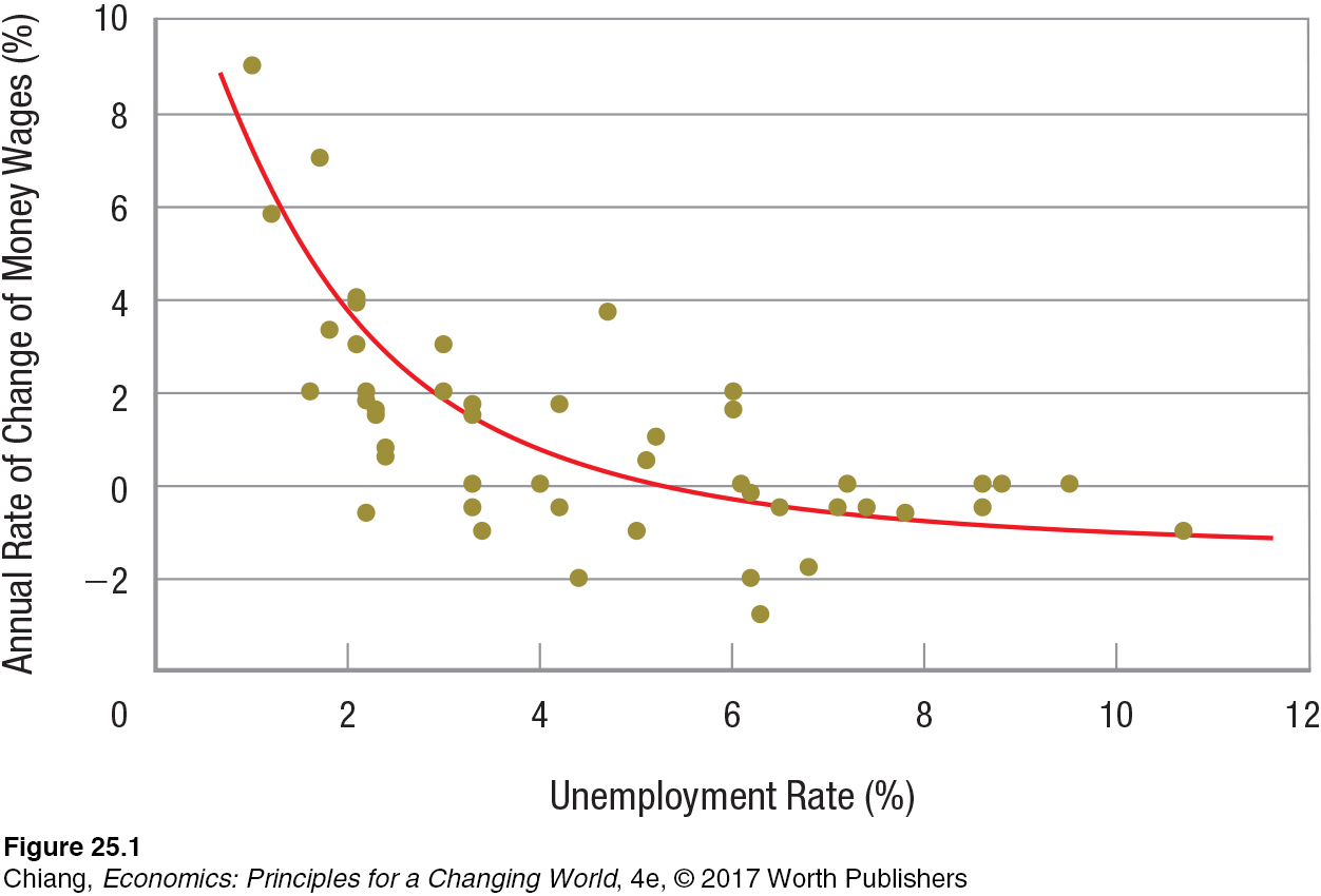
What explains this negative relationship between wages and unemployment? Labor costs or wages are typically a firm’s largest cost component. As the demand for labor rises, labor markets will tighten, making it difficult for employers to fill vacant positions. Hence, wages rise as firms bid up the price of labor to attract more workers. The opposite happens when labor demand falls: Unemployment rises and wages decline.

This relationship can be seen in specific industries that have seen spikes or downturns in employment. For example, demand for health care professionals increased in the past decade, reducing unemployment in the industry. Those who pursue a career in nursing, medicine, or other health-related fields saw their salaries increase relative to those in other careers. On the other hand, the collapse of the financial and housing sectors forced many realtors, loan specialists, and construction workers out of work. Those lucky enough to find work often made less than they did during the housing boom.

675

The market relationship between wages and unemployment will clearly affect prices. But worker productivity also plays an important role in determining prices.

Productivity, Prices, and Wages We might think that whenever wages rise, prices must also rise. Higher wages mean higher labor costs for employers—costs that businesses then pass along as higher prices. But this is not always the case. If worker productivity increases enough to offset the wage increase, then product prices can remain stable. The basic relationship among wages, prices, and productivity is

Inflation = Increase in Nominal Wages − Rate of Increase in Labor Productivity

For example, when wages increase by 5% and productivity increases by 3%, inflation is 2%. Given this relationship, the Phillips curve can be adapted to relate productivity to inflation and unemployment, as shown in Figure 2.

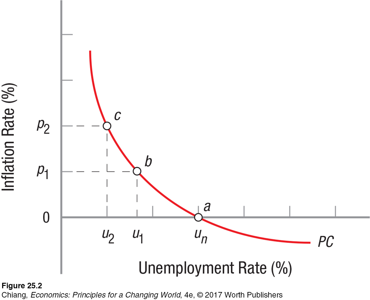
Notice that when the rates of change in productivity and wages are equal, inflation is zero (point a). This occurs at the natural rate of unemployment, the unemployment rate when inflationary pressures are nonexistent. Therefore, higher rates of productivity growth mean that for a given level of unemployment, inflation will be less (the Phillips curve would shift in toward the origin).

If policymakers want to use expansionary policy to reduce unemployment from u_n to u₁, then according to the curve shown in Figure 2, they must be willing to accept inflation of p₁. To reduce unemployment further to u₂ would raise inflation to p₂ as labor markets tightened and wages rose more rapidly.

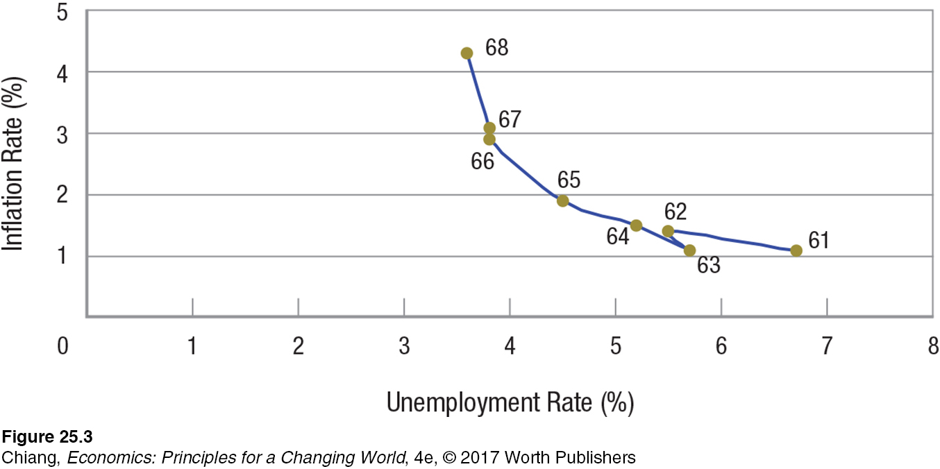
Figure 3 shows the Phillips curve for the United States during the 1960s. Notice the nearly smooth negative relationship between the two variables, much like that in the last two figures. As unemployment fell, inflation rose. This empirical relationship led policymakers to believe that the economy presents them with a menu of choices. By accepting a minor rise in inflation, they could keep unemployment low. Alternatively, by accepting a rise in unemployment, they could keep inflation near zero.

676

But just as policymakers were getting used to the ease of making policy by accepting moderate inflation in exchange for lower unemployment rates, the economy played a big trick on them. As Figure 4 shows, the entire Phillips curve began shifting outward during the early 1970s.

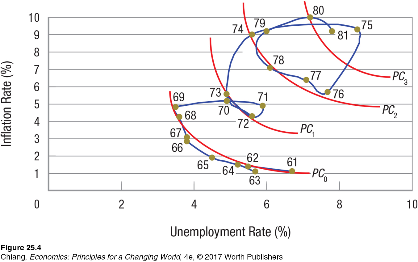
What looked to be an easy tradeoff between inflation and unemployment turned ugly. Unemployment rates that, in the 1960s, had been associated with modest inflation of 2% to 3% quickly began requiring twice that rate in the early 1970s. By the late 1970s, these same unemployment rates were generating annual inflation rates approaching double digits. The reason for these shifts turned out to be the oil supply shocks of the mid-1970s and the rising inflationary expectations that followed.

The Importance of Inflationary Expectations Workers do not work for the sake of earning a specific dollar amount, or a specific nominal wage. Rather, they work for the sake of earning what those wages will buy—for real wages. Consequently, when they bargain for wage increases, workers will take their past experiences with inflation into account.

Taking inflationary expectations into account, wage increases can be connected to unemployment and expected inflation by adding a variable, p^e, representing inflationary expectations, to the inflation equation introduced earlier:

677

Inflation = Increase in Nominal Wages − Rate of Increase in Labor Productivity + P^e

In other words, the same tradeoff between inflation and unemployment in the short-run Phillips curve existed as we saw before, but there is a unique tradeoff for each level of inflationary expectations.

For example, suppose there are no inflationary expectations, and productivity is growing at a 3% rate when the economy’s unemployment rate is 4%. In this scenario, if nominal wages increase by 5%, inflation would be 5% − 3% + 0% = 2%. However, if inflationary expectations (p^e) grow to, say, 4%, the Phillips curve will shift outward and the inflation rate now associated with 4% unemployment will be 5% − 3% + 4% = 6%.

Inflationary Expectations and the Phillips Curve Panel B of Figure 5 shows a Phillips curve augmented by inflationary expectations. The economy begins in equilibrium at full employment with zero inflation (point a in panel B). Panel A shows the aggregate demand and supply curves for this economy in equilibrium at point a. Note that the economy is producing at full employment output of Q_f, and this translates to the natural rate of unemployment, u_n, in panel B.

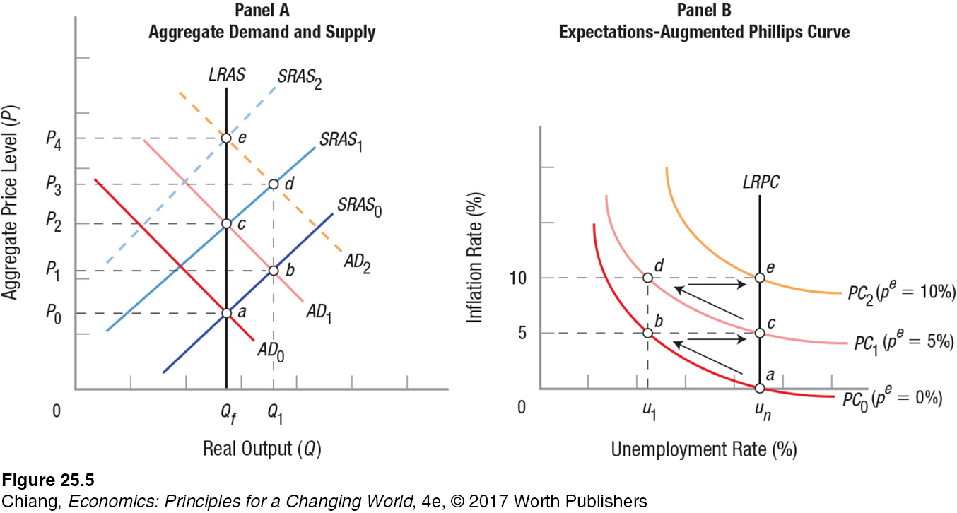
The Phillips curve in panel B is initially PC₀ (p^e = 0%). Thus, inflation is equal to zero and so are inflationary expectations (p^e).

Now assume, however, that policymakers are unhappy with the economy’s performance and want to reduce unemployment below u_n. Using expansionary policies, they shift aggregate demand in panel A from AD₀ to AD₁. This moves the economy to point b; real output and the price level rise, to Q₁ and P₁.

In panel B, meanwhile, the unemployment rate has declined to u₁ (point b), but inflation has risen to 5%. Workers had anticipated zero inflation; this unanticipated inflation means that real wages have fallen. Therefore, workers will begin asking for raises, and employers wanting to keep turnover at a minimum may well begin offering higher wages.

The Long-Run Phillips Curve The long-run Phillips curve (LRPC), shown in panel B of Figure 5 as the vertical line at full employment (unemployment = u_n), shows the long-term relationship between inflation and unemployment when the inflation rate and the expected inflation rate are equal. The LRPC is the Phillips curve counterpart to the vertical long-run aggregate supply curve (LRAS) in panel A.

678

Accelerating Inflation As nominal wages rise, the result in panel A is that, over time, the short-run aggregate supply curve shifts leftward to SRAS₁, thus moving the economy back to full employment at point c. In panel B, with inflation now running at 5%, the Phillips curve shifts outward to PC₁ (p^e = 5%). Workers, however, now expect 5% inflation, and the economy moves back to point c. Unemployment has moved back to its natural rate, but inflationary expectations have risen to 5%. The aggregate price level, meanwhile, has risen from P₀ to P₂, or 5%.

At this point, in order for policymakers to move the economy back to u₁ (or Q₁), they must repeat the process of expanding aggregate demand, only this time, the economy is starting from a higher Phillips curve because inflationary expectations are already elevated.

The implications of this analysis for fiscal and monetary policymakers who want to fine-tune the economy and keep unemployment below the natural rate are not pleasant. If policymakers want to keep unemployment below the natural rate, they must continually increase aggregate demand so that inflation will always exceed what is expected. Thus, policymakers must be willing to incur a permanently accelerating rate of inflation—hardly a popular idea.

In the late 1970s and early 1980s, oil price shocks and rising inflationary expectations caused both inflation and unemployment to rise, creating what economists call stagflation. Where under the original Phillips curve the conclusion was that rising unemployment would be met by falling inflation, the 1970s witnessed rising unemployment and rising inflation as the Phillips curve shifted outward. By 1980 inflation was over 10% and unemployment was over 7%.

679

Returning Inflation to Normal Levels To eliminate inflationary pressures when they arise, policymakers must be willing to curtail growth in aggregate demand and accept the resulting higher rates of unemployment for a certain transition period. How long it takes to reduce inflation and return to the natural rate of unemployment will depend on how rapidly the economy adjusts its inflationary expectations. Policymakers can speed this process along by ensuring their policies are credible, for instance, by issuing public announcements that are consistent with contractionary policies in both the monetary and fiscal realms.

To reduce inflationary expectations, policymakers must be willing to reduce aggregate demand and push the economy into a recession, increasing unemployment. As aggregate demand slumps, wage and price pressures will soften, reducing inflationary expectations. As these expectations decline, the Phillips curve shifts inward, back to a position with lower inflation at the natural rate of unemployment. How fast this occurs depends on the severity of the recession and the confidence the public has that policymakers are willing to stay the course.

The stagflation of the early 1980s required almost a decade to be resolved. Former Fed Chair Paul Volcker, who insisted on keeping interest rates high in the face of fierce public opposition, deserves much of the credit for this triumph over inflation.

This lesson about the importance of restraining monetary growth and focusing on stable prices was not lost on the next Fed Chair, Alan Greenspan. Throughout the 1990s, the Fed maintained a tight watch on inflation, which fell from around 4% to near 1%.

The importance of keeping inflation low has continued to influence policymaking today. As long as the threat of inflation remains low, policymakers have been willing to use expansionary policy to promote economic growth and reduce unemployment, exactly what the Phillips curve suggests would be effective. These policies assume that inflation expectations adjust with a noticeable lag, allowing some trade-off between inflation and unemployment to exist. Some economists, however, argue that consumers and businesses adapt their expectations so rapidly that their behavior tends to nullify much of policymakers’ actions, which we will discuss next.

Rational Expectations and Policy Formation The use of expectations in economic analysis is nothing new. Keynes believed that expectations are driven by emotions. He suggested that investors in the stock market will jump on board trends without attempting to understand the underlying market dynamics. Milton Friedman developed his model of expectations using what are known as adaptive expectations, whereby people are assumed to perform a simple extrapolation from past events. Workers, for example, are assumed to expect that past rates of inflation, averaged over some time period, will continue into the future. Adaptive expectations are represented by a backward-looking model of expectations, which contrasts with the rational expectations model.

680

In the rational expectations model developed by Robert Lucas, rational economic agents are assumed to make the best possible use of all publicly available information about what the future holds before making decisions. This does not mean that every individual’s predictions about the future will be correct. Those errors that do occur will be randomly distributed, such that the expectations of large numbers of people will average out to be correct.

Assume that the economy has been in an equilibrium state for several years with low inflation (2%) and unemployment (6%). In such a stable environment, the average person would expect the inflation rate to stay right about where it is indefinitely. But now assume that the Fed announces it is going to increase the rate of growth of the money supply significantly. Basic economic theory tells us that this action will translate into higher prices, bringing about higher future inflation rates. Knowing this, households and businesses will revise their inflationary expectations upward.

As this example shows, people do not rely only on past experiences to formulate their expectations of the future, but instead use all information available to them, including current policy announcements and other information that gives them reason to believe the future might hold certain changes. If adaptive expectations are backward-looking, rational expectations are forward-looking.

Policy Implications of Rational Expectations Do individuals and firms really form their future expectations as the rational expectations hypothesis suggests? If so, the implications for macroeconomic policy would be enormous; indeed, it could leave macroeconomic policy ineffective.

To illustrate, let us assume that the economy depicted in Figure 6 is operating at full employment at point a. Short-run aggregate supply curve SRAS₀ (P = 100) reflects current inflationary expectations. Suppose the Fed announces that it intends to increase the money supply.

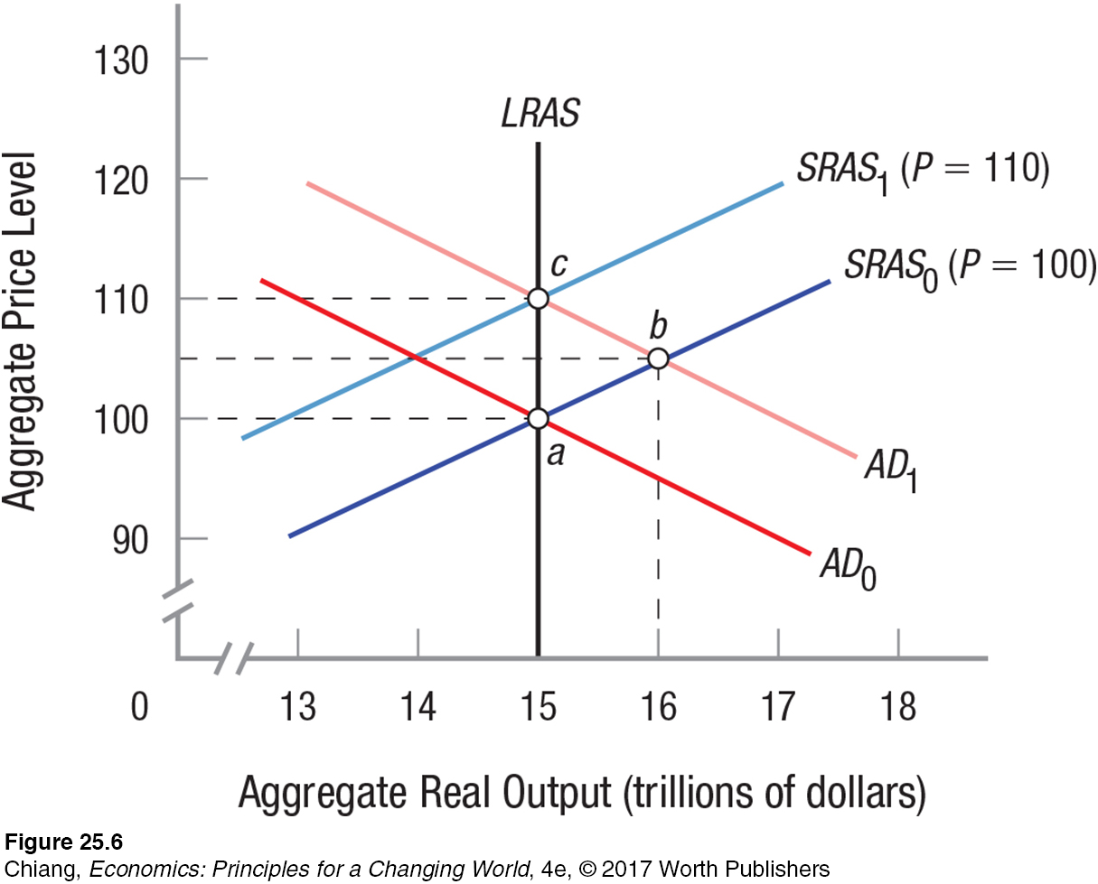
Expanding the money supply will shift aggregate demand from AD₀ to AD₁. This will increase the demand for labor and raise nominal wages. But what happens next?

Natural rate theorists, using adaptive expectations, would argue that workers will be fooled into thinking that the increase in money wages represents a real raise, thus driving output and employment up to $16 trillion (point b). After a time, however, workers will realize that real wages have not risen because prices have risen by at least as much as wages. Aggregate supply will then fall to SRAS₁ (P = 110) as price expectations climb and the economy gradually moves back to full employment at a higher price level (point c). In this scenario, the Fed’s policy succeeds in raising output and employment in the short term, but at the expense of a long-term rise in the cost of living.

681

Contrast this with the rational expectations model. When the Fed announces that it is going to increase the money supply, perfectly rational individuals and firms will listen to this information and immediately raise their inflationary expectations. In Figure 6, output will remain unchanged because the price level will rise immediately to 110. No one gets fooled into temporarily increasing output or employment, even though the increase in the money supply still drives up prices. Therefore, any announcement of a policy change will result in an immediate move to a new long-run equilibrium, leaving the short-term aspects of the policy change ineffective.

This suggests that if the Fed wants to use an increase in the money supply to raise output and employment in the short term, the only way it can do so is by not announcing its plans; it must essentially force individuals and firms to make decisions with substantially incomplete information.

A Critique of Rational Expectations To date, empirical assessments of the ineffectiveness of macroeconomic policy based on rational expectations have yielded mixed results. In general, these studies do not support the policy ineffectiveness proposition. That is, macroeconomic policies do have a real impact on the economy, and monetary policies are credited with keeping inflation low over the past three decades.

New Keynesian economists have taken a different approach to critiquing rational expectations theory. Both the adaptive and the rational expectations models assume that labor and product markets are highly competitive, with wages and prices adjusting quickly to expansionary or contractionary policies. The new Keynesians point out, however, that labor markets are often beset with imperfect information, and that efficiency wages often bring about short-term wage stickiness.

Imperfect information occurs when firms and workers do not have up-to-the-minute information on economic fluctuations due to timing lags, causing wages and prices to not react quickly. Efficiency wage theory disputes the notion that labor markets are like competitive commodity markets with equal prices. In other words, all labor is not equal. People need incentives to work hard, and paying workers an efficiency wage, or a wage above the market-clearing level, is one form of motivation to improve morale and productivity.

Imperfect information and efficiency wages suggest that wages and prices may be sticky because workers and firms are either unable or unwilling to make adjustments quickly to changes in the economy. This means that neither workers nor firms can react quickly to changes in monetary or fiscal policy. And this would give such policies a chance of a short-term impact.

Although the policy ineffectiveness proposition has not found significant empirical support, rational expectations as a concept has profoundly affected how economists approach macroeconomic problems. Nearly all economists agree that policy changes affect expectations, and that this affects the behavior of individuals and firms that potentially reduce the effectiveness of monetary and fiscal policy.

This section has considered two challenges to the effectiveness of macroeconomic policy. First, we looked at the Phillips curve, and showed that policies attempting to address unemployment could lead to inflation and a build-up in inflationary expectations. In other words, policymakers do not face an easy choice between rates of unemployment and rates of inflation. Second, we looked at rational expectations and showed how expectations could mitigate the effectiveness of policy.

In the next section, we now want to apply these concepts to macroeconomic issues that are important in our future: economic growth, jobs, debt, and globalization.

682