SUPPLY
The analysis of a market economy rests on two foundations: supply and demand. So far, we’ve covered the demand side of the market. Let’s focus now on the decisions businesses make regarding production numbers and sales. These decisions cause variations in product supply.
The Law of Supply: The Relationship Between Quantity Supplied and Price
supply The maximum amount of a product that sellers are willing and able to provide for sale over some time period at various prices, holding all other relevant factors constant (the ceteris paribus condition).
Supply is the maximum amount of a product that producers are willing and able to offer for sale at various prices, all other relevant factors being held constant. The quantity supplied will vary according to the price of the product.
What explains this relationship? As we saw in the previous chapter, businesses inevitably encounter rising opportunity costs as they attempt to produce more and more of a product. This is due in part to diminishing returns from available resources, and in part to the fact that when producers increase production, they must either have existing workers put in overtime (at a higher hourly pay rate) or hire additional workers away from other industries (again at premium pay).
Producing more units, therefore, makes it more expensive to produce each individual unit. These increasing costs give rise to the positive relationship between product price and quantity supplied to the market.
law of supply Holding all other relevant factors constant, as price increases, quantity supplied rises and as price declines, quantity supplied falls.
Unfortunately for producers, they can rarely charge whatever they would like for their products; they must charge whatever the market will permit. But producers can decide how much of their product to produce and offer for sale. The law of supply states that higher prices will lead producers to offer more of their products for sale during a given period. Conversely, if prices fall, producers will offer fewer products to the market. The explanation is simple: The higher the price, the greater the potential for higher profits and thus the greater the incentive for businesses to produce and sell more products. Also, given the rising opportunity costs associated with increasing production, producers need to charge these higher prices to increase the quantity supplied profitably.
Let’s return to our market for gaming apps. Why do programmers spend countless hours developing new gaming apps? Because they have an incentive to do so. Much like how consumers download more gaming apps when the price goes down, the opposite is true for suppliers. As the price rises, programmers are more willing to create new games, enhance existing games, and provide more server capacity (to ensure games operate smoothly) and technical support, all to increase the quantity of gaming apps supplied. Although gaming apps are not a physical good, the law of supply still applies. This is no different than an oil producer drilling for more oil when the price rises. In each case, producers respond to changes in price.
The Supply Curve
supply curve A graphical illustration of the law of supply, which shows the relationship between the price of a good and the quantity supplied.
Just as demand curves graphically display the law of demand, supply curves provide a graphical representation of the law of supply. The supply curve shows the maximum amounts of a product a producer will furnish at various prices during a given period of time. While the demand curve slopes down and to the right, the supply curve slopes up and to the right.1 This illustrates the positive relationship between price and quantity supplied: The higher the price, the greater the quantity supplied.
1 There are some exceptions to positively sloping supply curves. But for our purposes, we will ignore them for now.
Market Supply Curves
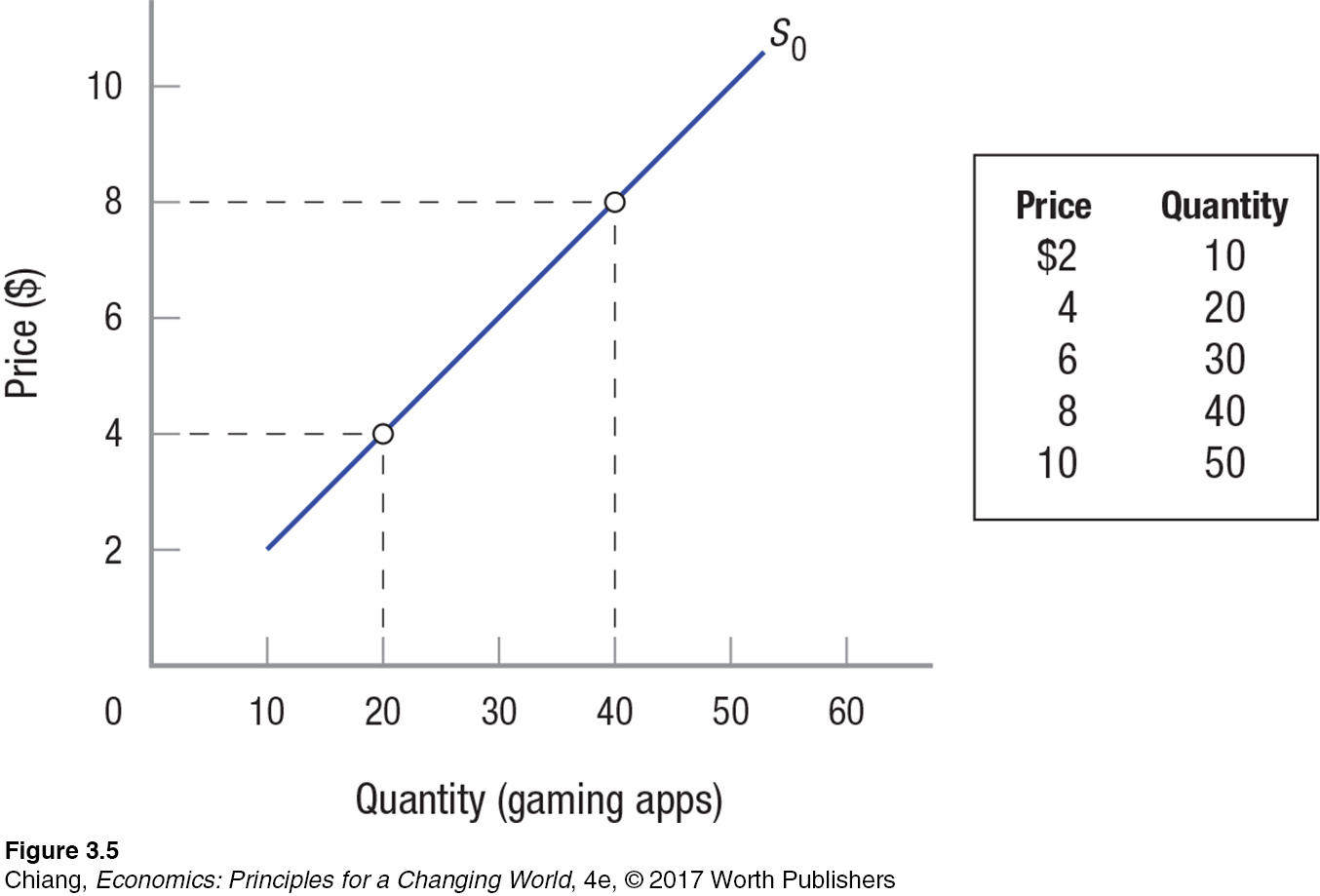
As with demand, economists are more interested in market supply than in the supplies offered by individual firms. To compute market supply, use the same method used to calculate market demand, horizontally summing the supplies of individual producers. A hypothetical market supply curve for gaming apps is depicted in Figure 5. The quantity of gaming apps that producers will offer for sale increases as the price of gaming apps rises. The opposite would happen if the price of gaming apps falls.
Determinants of Supply
determinants of supply Nonprice factors that affect supply, including production technology, costs of resources, prices of related commodities, expectations, number of sellers, and taxes and subsidies.
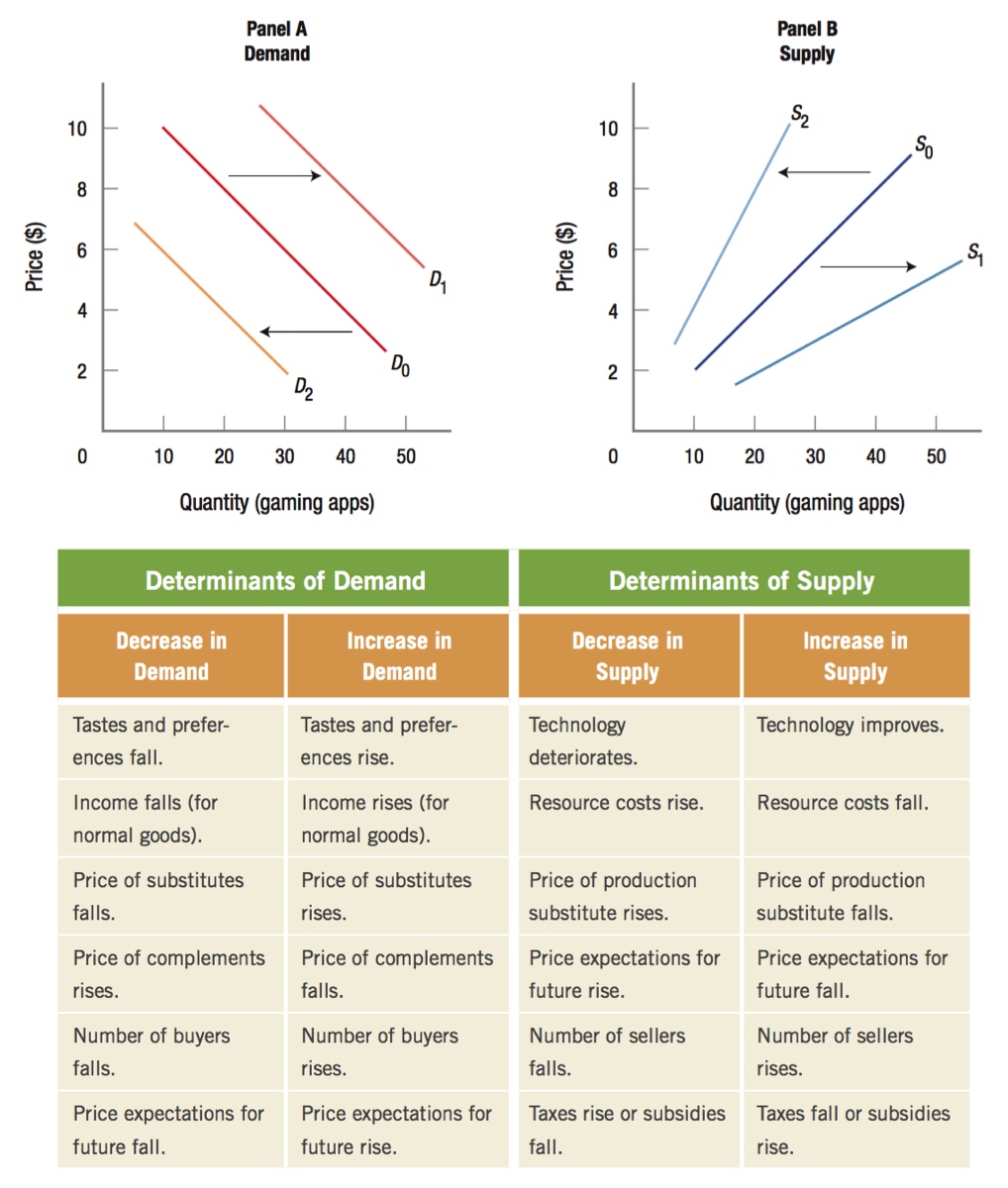
Like demand, several nonprice factors help to determine the supply of a product. Specifically, there are six determinants of supply: (1) production technology, (2) costs of resources, (3) prices of related commodities, (4) expectations, (5) the number of sellers (producers) in the market, and (6) taxes and subsidies.
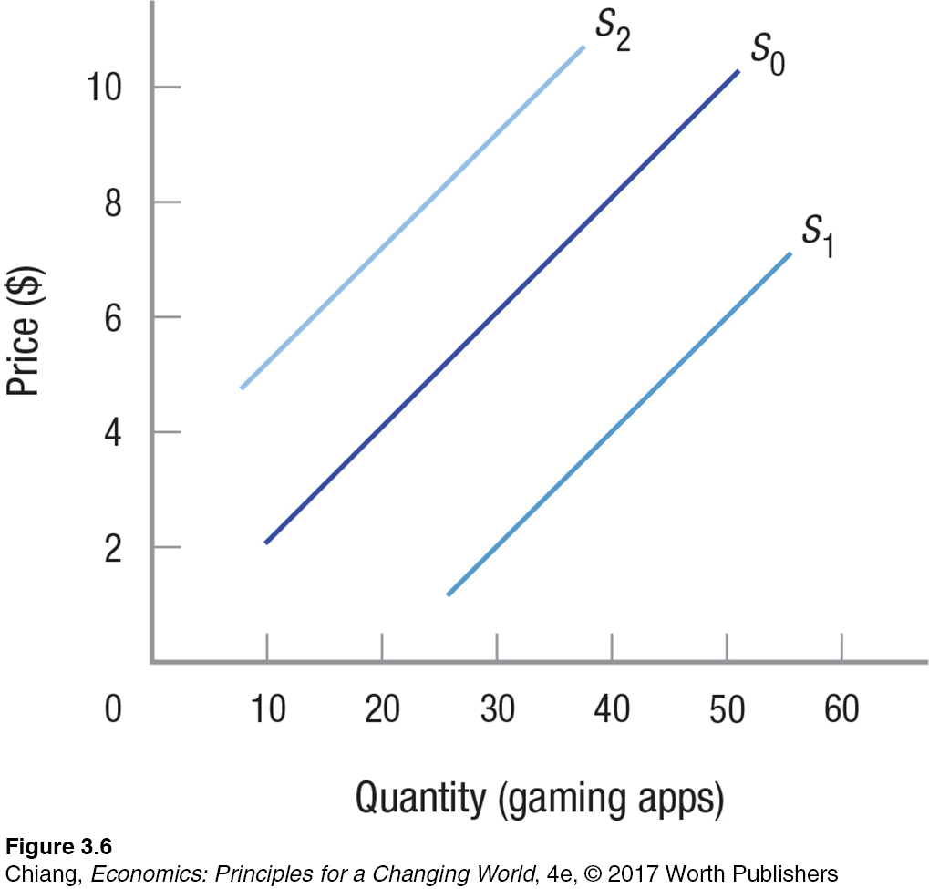
Production Technology Technology determines how much output can be produced from given quantities of resources. If a factory’s equipment is old and can produce only 50 units of output per hour, then no matter how many other resources are employed, those 50 units are the most the factory can produce in an hour. If the factory is outfitted with newer, more advanced equipment capable of turning out 100 units per hour, the firm can supply more of its product at the same price as before, or even at a lower price. In Figure 6, this would be represented by a shift in the supply curve from S0 to S1. At every single price, more would be supplied.
Technology further determines the nature of products that can be supplied to the market. A hundred years ago, the supply of computers on the market was zero because computers did not yet exist. More recent advances in microprocessing and miniaturization brought a wide array of products to the market that were not available just a few years ago, including mini-
Costs of Resources Resource costs clearly affect production costs and supply. If resources such as raw materials or labor become more expensive, production costs will rise and supply will be reduced (the supply curve shifts to the left, from S0 to S2 in Figure 6). The reverse is true if resource costs drop (the supply curve shifts to the right, from S0 to S1). The growing power of microchips along with their falling cost has resulted in cheap and plentiful electronics and computers. Nanotechnology—
However, when the cost of resources (such as oil and farm products) rise, the cost of products using those resources in their manufacture will go up, leading to the supply being reduced (the supply curve shifts leftward). If labor costs rise because immigration is restricted, this drives up production costs of California vegetables (fewer farmworkers) and software in Silicon Valley (fewer software engineers from abroad) and leads to a shift in the supply curve to the left in Figure 6.
Prices of Related Commodities Most firms have some flexibility in the portfolio of goods they produce. A vegetable farmer, for example, might be able to grow celery or radishes, or some combination of the two. Given this flexibility, a change in the price of one item may influence the quantity of other items brought to market. If the price of celery should rise, for instance, most farmers will start growing more celery. And since they all have a limited amount of land on which to grow vegetables, this reduces the quantity of radishes they can produce. Hence, in this case, the rise in the price of celery may well cause a reduction in the supply of radishes (the supply curve for radishes shifts leftward).
Expectations The effects of future expectations on market supplies can be confusing, but it need not be. When sellers expect prices of a good to rise in the future, they are likely to restrict their supply in the current period in anticipation of receiving higher prices in some future period. Examples include homes and stocks—
Eventually, if prices do rise in the next period, producers would increase the quantity supplied of the good; however, this would be due to the law of supply, not due to a shift of the supply curve. In other words, rising prices result in a movement along the supply curve. Only when producers anticipate a change in a future price, causing a reaction now, does supply shift.
Number of Sellers Everything else being held constant, if the number of sellers in a particular market increases, the market supply of their product increases. It is no great mystery why: Ten dim sum chefs can produce more dumplings in a given period than five dim sum chefs.
Taxes and Subsidies For businesses, taxes and subsidies affect costs. An increase in taxes (property, excise, or other fees) will shift supply to the left and reduce it. Subsidies are the opposite of taxes. If the government subsidizes the production of a product, supply will shift to the right and rise. A proposed new tax on expensive health care insurance plans may reduce supply (the tax is equivalent to an increase in production costs), while today’s subsidies to ethanol producers expand ethanol production.
Changes in Supply Versus Changes in Quantity Supplied
change in supply Occurs when one or more of the determinants of supply change, shown as a shift in the entire supply curve.
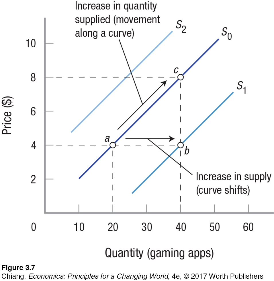
A change in supply results from a change in one or more of the determinants of supply; it causes the entire supply curve to shift. An increase in supply of a product, perhaps because advancing technology has made it cheaper to produce, means that more of the commodity will be offered for sale at every price. This causes the supply curve to shift to the right, as illustrated in Figure 7 by the shift from S0 to S1. A decrease in supply, conversely, shifts the supply curve to the left, since fewer units of the product are offered at every price. Such a decrease in supply is represented by the shift from S0 to S2.
change in quantity supplied Occurs when the price of the product changes, shown as a movement along an existing supply curve.
A change in supply involves a shift of the entire supply curve. In contrast, the supply curve does not move when there is a change in quantity supplied. Only a change in the price of a product can cause a change in the quantity supplied; hence, it involves a movement along an existing supply curve rather than a shift to an entirely different curve. In Figure 7, for example, an increase in price from $4 to $8 results in an increase in quantity supplied from 20 to 40 apps, represented by the movement from point a to point c along S0.
In summary, a change in supply is represented in Figure 7 by the shift from S0 to S1 or S2, which involves a shift in the entire supply curve. For example, an increase in supply from S0 to S1 results in an increase in supply from 20 gaming apps (point a) to 40 (point b) provided at a price of $4. More apps are provided at the same price. In contrast, a change in quantity supplied is shown in Figure 7 as a movement along an existing supply curve, S0, from point a to point c caused by an increase in the price of the product from $4 to $8.
As on the demand side, this distinction between changes in supply and changes in quantity supplied is crucial. It means that when a product’s price changes, only quantity supplied changes—
CHECKPOINT
SUPPLY
Supply is the quantity of a product producers are willing and able to put on the market at various prices, all other relevant factors being held constant.
The law of supply reflects the positive relationship between price and quantity supplied: The higher the market price, the more goods supplied, and the lower the market price, the fewer goods supplied.
As with demand, market supply is derived by horizontally summing the individual supplies of all of the firms in the market.
A change in supply occurs when one or more of the determinants of supply change.
The determinants of supply are production technology, the cost of resources, prices of related commodities, expectations about future prices, the number of sellers or producers in the market, and taxes and subsidies.
A change in supply is a shift in the supply curve. A shift to the right reflects an increase in supply, while a shift to the left represents a decrease in supply.
A change in quantity supplied is only caused by a change in the price of the product; it results in a movement along the existing supply curve.
QUESTIONS: At the end of the term, bookstores often increase the prices offered to students for their used textbooks in order to stock their shelves for the following term. Would an increase in the buyback price affect the supply or the quantity supplied of used textbooks? Suppose an unusually difficult professor leads to many students having to retake the course the next term. How might this affect the supply for used textbooks?
Answers to the Checkpoint questions can be found at the end of this chapter.
A higher textbook buyback price would entice more students to sell their textbooks instead of keeping them. Because the price of the offer has increased, it results in an increase in the quantity supplied of used textbooks. If, however, many students are forced to retake a class, they would likely not sell their textbooks; hence, the supply of used textbooks would shift to the left.