CHAPTER EXERCISES
Answers to the odd-numbered exercises appear in Appendix B.
Review Your Knowledge
13.01 Relationship tests look for a relationship between _______ variables in _______ group of cases.
13.02 A Pearson r measures the degree of _______ relationship between two _______ variables.
13.03 Measures of _______ quantify the degree of relationship between two variables.
13.04 If there’s a relationship between two variables, they are said to be _______.
13.05 If two variables are correlated, they vary together _______.
13.06 A Pearson r measures how much the points in a scatterplot fall in a _______ line.
13.07 If two variables are correlated, the relationship between them may be a _______ relationship.
13.08 Statisticians love to say that correlation _______ causation.
13.09 _______ are used to visualize the relationship between two interval/ratio variables.
13.10 If there is a cause-and-effect relationship between two variables, then they are _______. But, if two variables are correlated, there is not necessarily a _______ relationship between them.
13.11 The two variables in a correlation are usually labeled as _______ and _______.
13.12 The predictor variable in a correlation is the one that is viewed as _______ the other variable.
13.13 The dots fall in a _______ for a scatterplot showing no linear relationship between two normally distributed variables.
13.14 The strength of relationship, in a scatterplot, is determined by how well the points form a _______.
13.15 If the points in a scatterplot form a horizontal line, then r is _______.
13.16 Making a scatterplot using z scores instead of raw scores does / does not change the shape of the scatterplot.
13.17 In a perfect correlation, if a case has a z score of .75 for X, then its z score on Y is _______.
13.18 By the definitional formula for Pearson r, r is the _______ of multiplied-together pairs of _______.
13.19 A correlation coefficient is a number that _______ the strength of the relationship between _______.
13.20 If there is no linear relationship, then r = _______.
13.21 If r = .45, the relationship is _______ than if r = .70.
13.22 An r of _______ or _______ indicates a perfect linear relationship.
13.23 If r ranges from .01 to 1.00, the direction of the relationship is _______.
13.24 X and Y have an inverse relationship. As scores on X go up, scores on Y go _______.
13.25 An _______ is a score that falls far away from other scores.
13.26 An outlier can _______ the value of a correlation.
13.27 If the range of a variable is _______, then the full range of the variable is present in the sample.
13.28 A deflated value of a correlation can be caused by a _______.
13.29 The assumption that the sample is a random sample can / cannot be violated.
13.30 The linearity assumption is tested by making a _______.
13.31 The population value of a correlation is represented by the Greek letter _______.
13.32 The null and alternative hypotheses are statements about the _______ value of the correlation.
13.33 A nondirectional null hypothesis says there is _______ relationship in the population between X and Y.
13.34 The alternative hypothesis for a two-tailed test says there is _______ relationship in the population between X and Y, but it doesn’t state the _______ of the relationship.
13.35 If a researcher is doing a one-tailed test, first determine the _______ hypothesis.
13.36 If the alternative hypothesis is ρ < 0, then the researcher believes the relationship between X and Y is direct / inverse
13.37 If the null hypothesis for a two-tailed test is true, then the sampling distribution of r ranges from _______ to _______ and is centered on _______.
13.38 If the hypotheses are nondirectional, then one is completing a _______-tailed test.
13.39 By setting alpha at .05, one is willing to make a Type _______ error 5% of the time.
13.40 Finding rcv depends on the number of tails in the test, alpha, and _______.
13.41 If r ≥ rcv, then _______ the null hypothesis.
13.42 APA says a correlation should be reported as _______, not 0.45.
13.43 When getting ready to interpret Pearson r results, it is helpful to review the _______.
13.44 The first question addressed in interpretation is _______.
13.45 To decide if the null hypothesis is rejected, implement the _______ developed in Step 4 of the hypothesis-testing procedure.
13.46 If the null hypothesis is not rejected, the results are said to be _______ significant.
13.47 If APA format says r(8) = –.23, p > .05, then N = _______.
13.48 If APA format says r(8) = –.23, p > .05, then the results were _______ significant.
13.49 If the null hypothesis is rejected and r is –.23, then one can conclude that there is a _______ relationship between X and Y, also known as an _______ relationship.
13.50 If the relationship between X and Y is a direct one, then cases with high scores on X are likely to have _______ scores on Y.
13.51 If the null hypothesis is not rejected, _______ evidence exists to say that there is a _______ between X and Y.
13.52 If a result is not statistically significant, then there is a possibility of a _______ error.
13.53 _______ reveals the percentage of variability in one variable that is accounted for by the other variable.
13.54 As r2 gets closer to _______%, the effect is considered stronger.
13.55 If a relationship is perfect, r2 is _______%.
13.56 Cohen considers an r2 of _______% or greater to be a large effect.
13.57 The confidence interval for a Pearson correlation coefficient gives the range within which _______ likely falls.
13.58 When transforming a confidence interval from zr units to r units, make sure to maintain the _______ of the zr units.
13.59 If the confidence interval captures zero, the null hypothesis was / was not rejected.
13.60 If the confidence interval is wide, one is likely to recommend _______ of the study with a larger _______.
13.61 Power is the probability of __________ the null hypothesis when the null hypothesis should /should not be rejected.
13.62 Statisticians like power to be at least __________.
13.63 If power = .46, the probability of Type II error = __________.
13.64 To have an 80% chance of rejecting the null hypothesis if r = .60, one should have about ________ cases.
13.65 Correlation is not causation. A technique for dealing with a confounding variable is called ________.
13.66 A partial correlation mathematically ________________ the effect of a third variable.
Apply Your Knowledge
Making scatterplots
13.67 Given these data, make a scatterplot:
| Case | 1 | 2 | 3 | 4 | 5 | 6 | 7 | 8 | 9 | 10 | 11 | 12 | 13 | 14 | 15 |
| X | 5 | 8 | 12 | 16 | 19 | 22 | 26 | 31 | 12 | 25 | 18 | 6 | 30 | 22 | 9 |
| Y | 5 | 10 | 13 | 12 | 9 | 4 | 5 | 11 | 13 | 6 | 10 | 6 | 8 | 6 | 8 |
13.68 Given these data, make a scatterplot:
| Case | 1 | 2 | 3 | 4 | 5 | 6 | 7 | 8 | 9 | 10 | 11 | 12 | 13 | 14 | 15 |
| X | 44 | 46 | 48 | 47 | 49 | 50 | 48 | 49 | 52 | 52 | 53 | 54 | 54 | 55 | 56 |
| Y | 29 | 25 | 28 | 34 | 26 | 30 | 32 | 36 | 27 | 37 | 24 | 31 | 34 | 25 | 30 |
Select the appropriate test from among a single-sample z test; single-sample t test; independent-samples t test; paired-samples t test; between-subjects, one-way ANOVA; one-way, repeated-measures ANOVA; between-subjects, two-way ANOVA; and Pearson r.
13.69 “People who wear hats in the wintertime are compared to those who don’t wear hats in terms of how many days they suffer from a headcold. Does wearing a hat make a difference?” What test should be used to decide?
13.70 “People are measured, on an interval scale, to determine how fair-skinned they are. A dermatologist then examines them to see how many suspicious moles they have in order to determine if fairness of skin relates to the number of suspicious moles.” What statistical test should she use to answer this question?
13.71 “A behavioral therapist had patients with spider phobias rate the level of their fear on an interval-level scale. He then asked the spider phobics to enter a room with a spider in a cage and come as close to the spider as they felt comfortable. He measured the distance in feet. Do people with more self-reported fear stay a greater distance away?” What statistical test should the therapist use to find out?
13.72 “A kindergarten teacher classifies students as coloring inside the lines or coloring outside the lines. Years later, he uses police records to determine how many driving violations each former student has had. Is there a relationship between following the rules in kindergarten and following them on the highway?” What statistical test should be used?
Checking assumptions
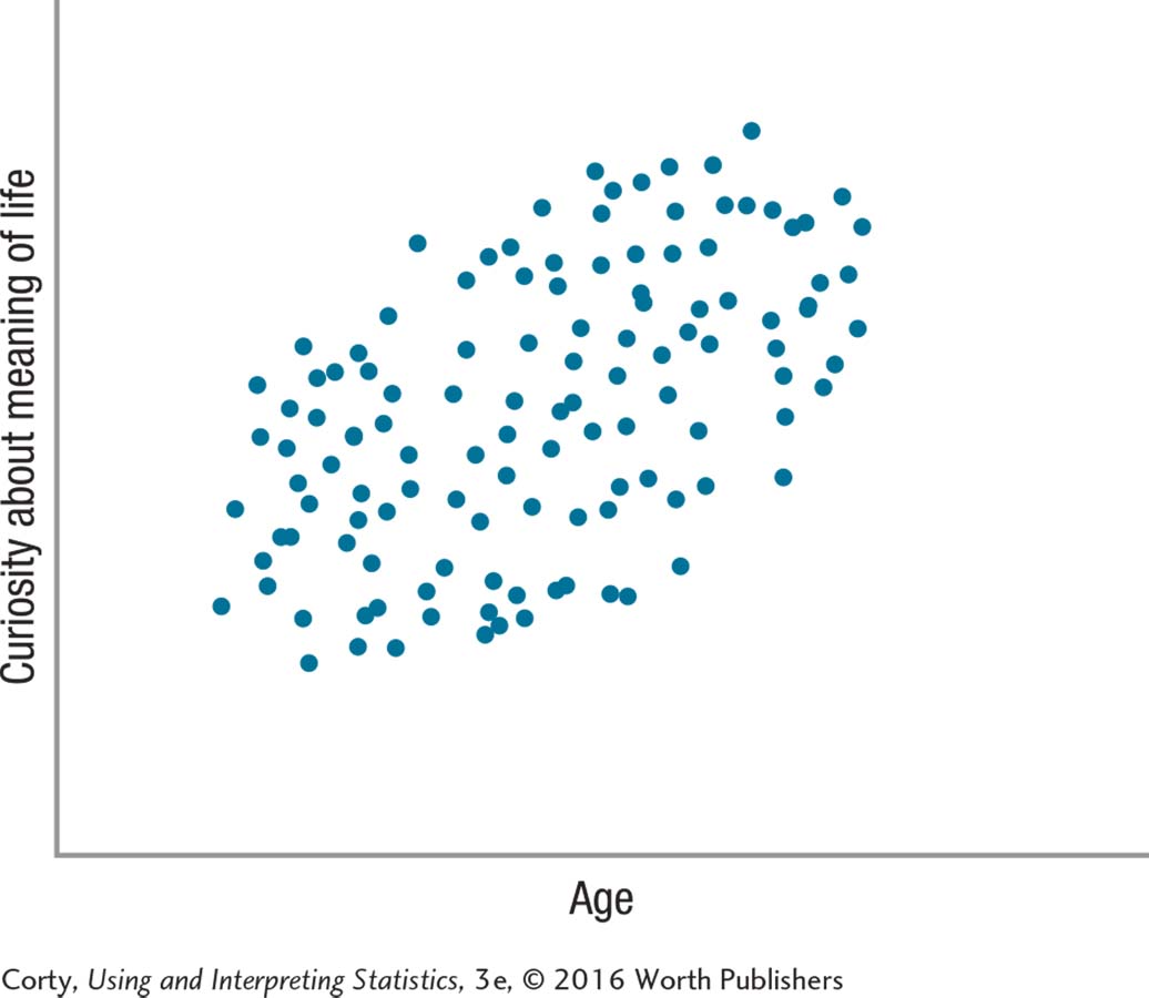
13.73 A philosopher wanted to see if curiosity about the meaning of life had any correlation, either positive or negative, with the age of college students and planned to use a Pearson r on her data. She obtained a random sample of 250 undergraduate students at the college where she taught and administered the Degree of Curiosity About the Meaning of Life Scale (an interval-level scale) to each one. Here is the scatterplot of her results. (a) Check the assumptions and (b) decide if she can proceed with the planned Pearson r.
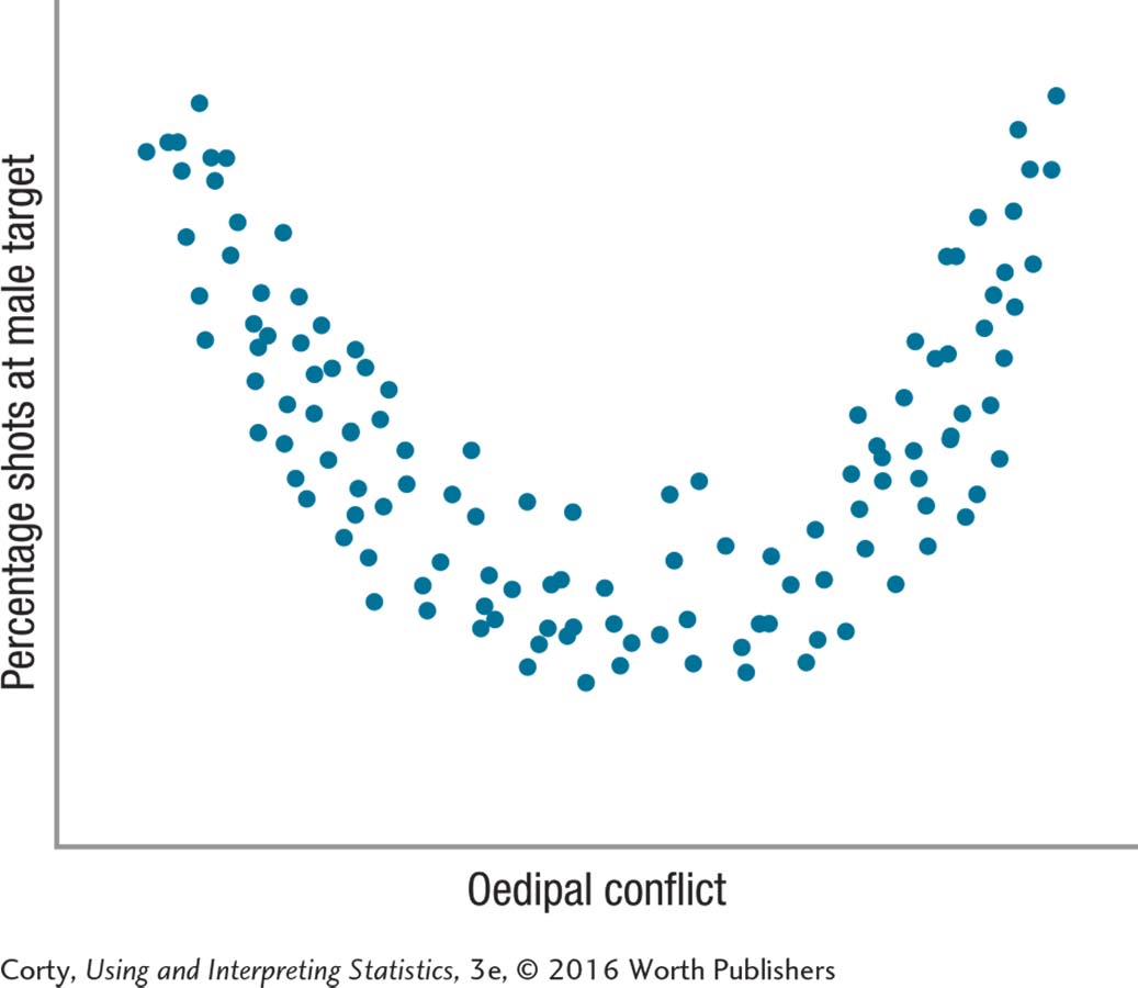
13.74 A psychodynamic psychologist used an interval-level scale to measure the degree of Oedipal conflict in a large sample of elementary age boys. He then had each one, by himself, play a target-shooting game where the boy had equal opportunity to shoot at male and female targets. The psychologist calculated the percentage of time the male target was shot at and considered that a measure of degree of hostility toward father figures. He wanted to use a Pearson r to examine the relationship, if any and if positive or negative, between Oedipal conflict and hostility toward father figures. Here is the scatterplot of the results. (a) Check the assumptions and (b) decide if he can proceed with the planned Pearson r.
Listing hypotheses
13.75 Assuming that a Pearson r can be used to analyze the data in Exercise 13.74, list the hypotheses.
13.76 A sleep specialist believes that the more caffeine a person consumes per day, the more episodes of restless sleep that person experiences. What are her null and alternative hypotheses?
Calculating degrees of freedom
13.77 What is df for a Pearson r if N = 63?
13.78 What is df for a Pearson r if N = 212?
Finding rcv
13.79 Given a two-tailed test with α = .05 and df = 7, what is rcv?
13.80 Given a two-tailed test with α = .05 and df = 27, what is rcv?
13.81 Given a one-tailed test, α = .05, N = 33, and H1: ρ > 0, what is rcv?
13.82 Given a one-tailed test, α = .05, N =33, and H1: ρ < 0, what is rcv?
Setting the decision rule
13.83 If rcv = ±.438, what is the decision rule?
13.84 If rcv = ±.554, what is the decision rule?
13.85 If rcv = ±.200, draw the sampling distribution of r and label the rare and common zones.
13.86 If rcv = ±.404, draw the sampling distribution of r and label the rare and common zones.
Calculating deviation scores
13.87 Given MX = 9.00 and MY = 5.00, calculate deviation scores for X and Y.
| X | Y |
| 12 | 6 |
| 8 | 3 |
| 7 | 6 |
13.88 Given MX = 16.33 and MY = 14.00, calculate deviation scores for X and Y.
| X | Y |
| 18 | 7 |
| 8 | 11 |
| 23 | 24 |
Multiplying deviation scores
13.89 (a) Multiply together the pairs of deviation scores and (b) sum the products.
| X | Y | X Deviation Scores | Y Deviation Scores |
| 10 | 65 | –2.33 | 11.67 |
| 18 | 55 | 5.67 | 1.67 |
| 9 | 40 | –3.33 | –13.33 |
| M = 12.33 | M = 53.33 |
13.90 (a) Multiply together the pairs of deviation scores and (b) sum the products.
| X | Y | X Deviation Scores | Y Deviation Scores |
| 540 | 115 | 36.67 | 11.33 |
| 510 | 88 | 6.67 | –15.67 |
| 460 | 108 | –43.33 | 4.33 |
| M = 503.33 | M = 103.67 |
Squaring deviation scores
13.91 (a) Square the deviation scores and (b) sum the squared scores.
| X | Y | X Deviation Scores | Y Deviation Scores | Product of Deviation Scores | Squared X Deviation Scores | Squared Y Deviation Scores |
| 21 | 110 | –4.33 | 10.67 | –46.20 | ||
| 38 | 90 | 12.67 | –9.33 | –118.21 | ||
| 17 | 98 | –8.33 | –1.33 | 11.08 | ||
| M = 25.33 | M = 99.33 | Σ = –153.33 |
13.92 (a) Square the deviation scores and (b) sum the squared scores.
| X | Y | XDeviation Scores | YDeviation Scores | Product of Deviation Scores | Squared X Deviation Scores | Squared Y Deviation Scores |
| 230 | 55 | –10.00 | –8.33 | 83.30 | ||
| 210 | 68 | –30.00 | 4.67 | –140.10 | ||
| 280 | 67 | 40.00 | 3.67 | 146.80 | ||
| M = 240.00 | M = 63.33 | Σ = 90.00 |
Multiplying sums of squares
13.93 (a) Multiply together the two sums of the squared deviation scores and (b) find the square root of that product.
| X | Y | X Deviation Scores | YDeviation Scores | Product of Deviation Scores | Squared X Deviation Scores | Squared Y Deviation Scores |
| 88 | 23 | 1.67 | –5.00 | –8.35 | 2.79 | 25.00 |
| 93 | 28 | 6.67 | 0.00 | 0.00 | 44.49 | 0.00 |
| 78 | 33 | –8.33 | 5.00 | –41.65 | 69.39 | 25.00 |
| M = 86.33 | M = 28.00 | Σ = –50.00 | Σ = 116.67 | Σ = 50.00 |
13.94 (a) Multiply together the two sums of the squared deviation scores and (b) find the square root of that product.
| X | Y | X Deviation Scores | Y Deviation Scores | Product of Deviation Scores | Squared X Deviation Scores | Squared Y Deviation Scores |
| 780 | 560 | –62.67 | –33.33 | 2,088.79 | 3,927.53 | 1,110.89 |
| 848 | 740 | 5.33 | 146.67 | 781.75 | 28.41 | 21,512.09 |
| 900 | 480 | 57.33 | –113.33 | –6,497.21 | 3,286.73 | 12,843.69 |
| M = 842.67 | M = 593.33 | Σ = –3,626.67 | Σ = 7,242.67 | Σ = 35,466.67 |
Calculating r
13.95 Given and Σ[(X – Mx)(Y – My)] = 255.70 and 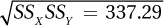 , calculate r.
13.96 Given and Σ[(X – Mx)(Y – My)] = –564.32 and  , calculate r.
13.97 Given the information in this table, calculate r:
| X | Y | X Deviation Scores | Y Deviation Scores | Product of Deviation Scores | Squared X Deviation Scores | Squared Y Deviation Scores |
| 7.6 | 5.6 | –0.90 | 0.11 | –0.10 | 0.81 | 0.01 |
| 6.8 | 7.4 | –1.70 | 1.91 | –3.25 | 2.89 | 3.65 |
| 9.0 | 4.8 | 0.50 | –0.69 | –0.35 | 0.25 | 0.48 |
| 9.0 | 4.0 | 0.50 | –1.49 | –0.75 | 0.25 | 2.22 |
| 11.0 | 3.4 | 2.50 | –2.09 | –5.23 | 6.25 | 4.37 |
| 8.0 | 3.5 | –0.50 | –1.99 | 1.00 | 0.25 | 3.96 |
| 7.6 | 7.8 | –0.90 | 2.31 | –2.08 | 0.81 | 5.34 |
| 8.0 | 6.6 | –0.50 | 1.11 | –0.56 | 0.25 | 1.23 |
| 8.7 | 7.8 | 0.20 | 2.31 | 0.46 | 0.04 | 5.34 |
| 9.3 | 4.0 | 0.80 | –1.49 | –1.19 | 0.64 | 2.22 |
| M = 8.50 | M = 5.49 | Σ = –12.03 | Σ = 12.44 | Σ = 28.81 |
13.98 Given the information in this table, calculate r:
| X | Y | X Deviation Scores | Y Deviation Scores | Product of Deviation Scores | Squared X Deviation Scores | Squared Y Deviation Scores |
| –2 | –3 | –1.80 | –2.60 | 4.68 | 3.24 | 6.76 |
| –2 | 2 | –1.80 | 2.40 | –4.32 | 3.24 | 5.76 |
| 5 | –5 | 5.20 | –4.60 | –23.92 | 27.04 | 21.16 |
| –6 | 3 | –5.80 | 3.40 | –19.72 | 33.64 | 11.56 |
| 2 | –6 | 2.20 | –5.60 | –12.32 | 4.84 | 31.36 |
| –2 | 0 | –1.80 | 0.40 | –0.72 | 3.24 | 0.16 |
| 0 | 1 | 0.20 | 1.40 | 0.28 | 0.04 | 1.96 |
| –1 | –1 | –0.80 | –0.60 | 0.48 | 0.64 | 0.36 |
| 2 | 2 | 2.20 | 2.40 | 5.28 | 4.84 | 5.76 |
| 2 | 3 | 2.20 | 3.40 | 7.48 | 4.84 | 11.56 |
| M = –0.20 | M = –0.40 | Σ = –42.80 | Σ = 85.60 | Σ = 96.40 |
Implementing the decision rule for a two-tailed test
13.99 rcv = ±.217 and r = –.17. State (a) whether the null hypothesis was rejected, and (b) whether or not the results are statistically significant.
13.100 rcv = ±.301 and r = –.31. State (a) whether the null hypothesis was rejected, and (b) whether or not the results are statistically significant.
Writing APA format with α = .05, two-tailed
13.101 Given df = 20 and r = –.67, write the results in APA format.
13.102 Given df = 87 and r = –.18, write the results in APA format.
Interpreting APA format
13.103 If r(18) = –.50, p < .05, (a) was the null hypothesis rejected, and (b) were the results statistically significant?
13.104 If r(80) = –.18, p > .05, (a) was the null hypothesis rejected, and (b) were the results statistically significant?
13.105 If r(24) = .36, p > .05, (a) what conclusion can be drawn about the existence of a relationship between X and Y in the population? (b) Comment on the direction of the relationship in the population.
13.106 If r(30) = .40, p < .05, (a) what conclusion can be drawn about the existence of a relationship between X and Y in the population? (b) Comment on the direction of the relationship in the population.
Calculating r2
13.107 If r = .32, (a) calculate r squared and (b) classify the effect as small, medium, or large.
13.108 If r = –.05, (a) calculate r squared and (b) classify the effect as small, medium, or large.
Transforming r to zr
13.109 If r = –.46, what is zr?
13.110 If r = .33, what is zr?
Calculating sr
13.111 If N = 81, what is sr?
13.112 If N = 36, what is sr?
Finding the confidence interval in zr units
13.113 If zr = –0.34 and sr = .24, what is the 95% confidence interval for ρ in zr units?
13.114 If zr = 0.87 and sr = .08, what is the 95% confidence interval for ρ in zr units?
13.115 If r = .54 and N = 45, what is the 95% confidence interval for ρ in zr units?
13.116 If r = –.28 and N = 144, what is the 95% confidence interval for ρ in zr units?
Transforming a confidence interval back into r units
13.117 If a 95% confidence interval for ρ in zr units ranges from –0.85 to –0.41, what is it in r units?
13.118 If a 95% confidence interval for ρ in zr units ranges from –1.52 to –0.26, what is it in r units?
Interpreting confidence intervals
13.119 A 95% confidence interval for ρ ranges from –.09 to .93.
Was the null hypothesis rejected?
Were the results statistically significant?
Could the relationship between X and Y in the population be weak?
How sure is one about the population value of the correlation?
13.120 A 95% confidence interval for ρ ranges from .61 to .70.
Was the null hypothesis rejected?
Were the results statistically significant?
Could the relationship between X and Y in the population be weak?
How sure is one about the population value of the correlation?
Calculating power, β, and N
13.121 If r = .66 and N = 72, what is its power and what is β?
13.122 If r = .45 and N = 17, what is its power and what is β?
13.123 How many cases should one have to have in order to have adequate power if r = .28.
13.124 How many cases should one have to have in order to have adequate power if r = 57.
Completing an interpretation
13.125 A kinesiologist and a psychologist collaborated on a study to investigate the relationship between exercise and mental health. They obtained a random sample of 1,002 American men. They administered an interval-level mental health scale to each man and measured how many minutes of aerobic exercise each got per week. (On both measures, higher scores are better.) No assumptions were violated for the Pearson r and they found r(1,000) = .36, p <.05. r2 was 12.96% and the 95% confidence interval ranged from .31 to .41. Complete a four-point interpretation.
13.126 An economist wanted to investigate the relationship between the personality variable of conscientiousness and saving money. She obtained a random sample of 502 white-collar workers. She had each worker complete a personality inventory on which higher scores indicated more conscientiousness. She also asked each worker to report the percentage of income saved each month. No assumptions were violated for the Pearson r and she found r(500) = .11, p < .05. r2 was 1.21% and the 95% confidence interval ranged from .03 to .19. Complete a four-point interpretation.
Calculating a partial correlation
13.127 Using N = 32, rXY = .28, rXZ = .20, and rYZ = .22, calculate rXY–Z.
13.128 Using N = 108, rXY = .63, rXZ = .66, and rYZ = .45, calculate rXY–Z.
Interpreting partial correlations
13.129 Dr. Jones investigates the relationship between intelligence and number of absences from school in high school students. She finds a statistically significant relationship of –.33: those with higher IQs have fewer absences. She then partials out socioeconomic status and the correlation becomes –.13. Because her sample size was large, the correlation is still statistically significant. Interpret the results.
13.130 Dr. Atropos examines the correlation between years of sun exposure and healthiness of the skin. He finds a statistically significant correlation of –.44: the more years of sun exposure, the less healthy the skin. Thinking that more educated people might be more aware of the risk of melanoma, he partials out years of education and finds rXY–Z = –.41. Interpret the results.
Completing all six steps of hypothesis testing
13.131 A dentist wanted to determine if a relationship existed between childhood fluoride exposure and cavities. She took a sample of adults in her practice and counted how many cavities each person had in his or her permanent teeth. She also determined how many years of childhood each person was exposed to tap water with fluoride. The minimum value on this variable was 0 and the maximum was 18. Here are the data she collected:
| Case 1 | Case 2 | Case 3 | Case 4 | Case 5 | Case 6 | |
| X (years of fluoride) | 0 | 18 | 2 | 12 | 3 | 10 |
| Y (number of cavities) | 10 | 1 | 7 | 3 | 5 | 4 |
13.132 A sociologist wanted to see if there was a relationship between a family’s educational status and the eliteness of the college that their oldest child attended. She measured educational status by counting how many years of education beyond high school the parents had received. In addition, she measured the eliteness of the school by its yearly tuition, in thousands (e.g., 5 = $5,000). She obtained a random sample of 10 families.
| 1 | 2 | 3 | 4 | 5 | 6 | 7 | 8 | 9 | 10 | |
| Years post-HS education | 0 | 7 | 8 | 8 | 4 | 5 | 12 | 17 | 8 | 2 |
| Yearly tuition | 12 | 26 | 33 | 18 | 20 | 7 | 15 | 38 | 41 | 5 |
Expand Your Knowledge
13.133 A researcher has completed a study and found r(28) = –.23, p > .05. What should she conclude about the direction of the relationship between X and Y in the population?
13.134 Dr. Smith had a sample of 19 cases, violated no assumptions, and calculated r = .46. She was conducting a two-tailed test with α =.05. r2 = 21.16% and the 95% CI ranges from .01 to .76. What type of error does she need to worry about?
Type I
Type II
Both Type I and Type II
Neither Type I nor Type II
Type II because it is a two-tailed test. It would be Type I if the test was one-tailed.
There’s not enough information to tell.
13.135 Dr. Jones had 92 cases, violated no assumptions, conducted a two-tailed test with α = .05, and calculated r = –1.26. Which are accurate descriptions of the relationship between X and Y? (Select as many as are appropriate.)
It is an inverse relationship.
It is a direct relationship.
It is a curvilinear relationship.
It is a linear relationship.
It is not significantly different from zero.
It is significantly different from zero
There was some error in calculating r.
13.136 The owner of a hair salon is curious about the relationship between the amount of hair cut and the amount of money earned by the stylists. At the end of a randomly selected day, she weighed the amount of hair around the chairs of her eight stylists and counted their earnings. Below are the data she collected. Analyze them using the six-step hypothesis-testing procedure.
| 1 | 2 | 3 | 4 | 5 | 6 | 7 | 8 | |
| Pounds of hair | 1 | 10 | 2 | 8 | 4 | 7 | 5 | 6 |
| Earnings | 195 | 223 | 150 | 165 | 104 | 130 | 60 | 100 |
13.137 How many cases should one have in order to have adequate power to use a Pearson r to find a small effect? Medium effect? Large effect?
13.138 Rebekah used an independent-samples t test to compare a control group to an experimental group. She had 284 cases and found t = 4.38. Was her study underpowered?
SPSS
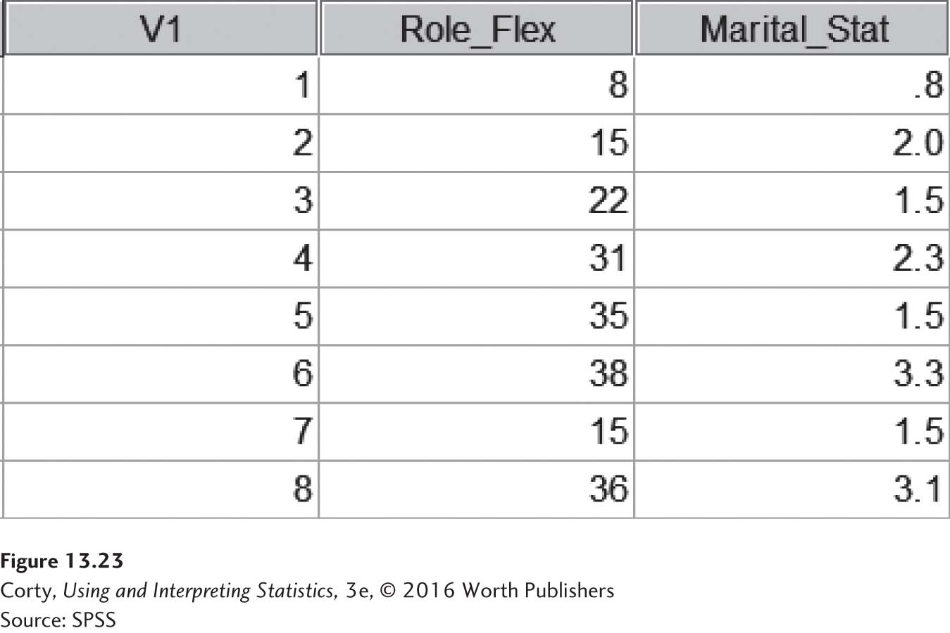
The data for a Pearson correlation coefficient in SPSS should be arranged with each variable in a column and each case in a row. Figure 13.23 shows how the data for the eight cases in Dr. Paik’s marital satisfaction study would look.
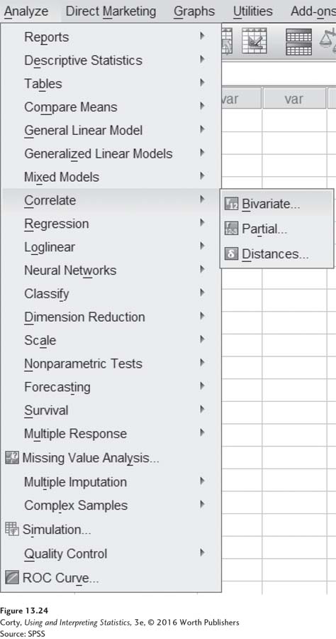
The commands for a Pearson r in SPSS are found under “Analyze,” then “Correlate,” and finally “Bivariate,” as shown in Figure 13.24.
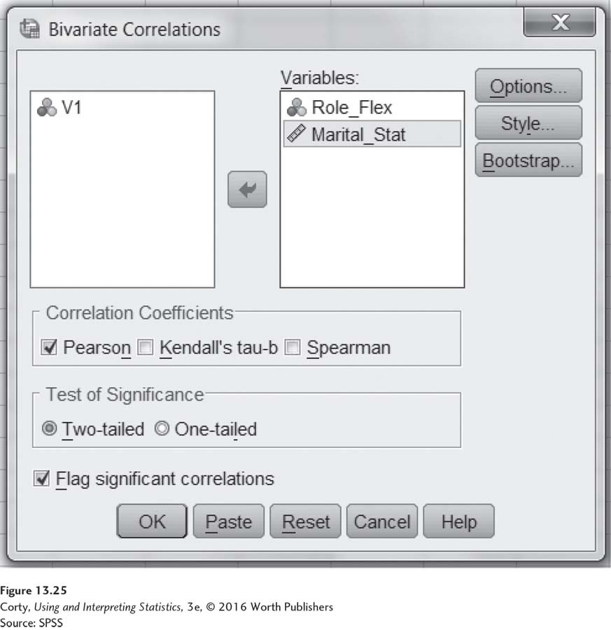
Clicking on “Bivariate” opens the menu seen in Figure 13.25. Highlight each of the variables to correlate and use the arrow button to move them over to the box labeled “Variables.” In Figure 13.25, note that the SPSS default options include Pearson r, a two-tailed test, and flagging significant correlations.
The SPSS output is shown in Figure 13.26. SPSS does each correlation twice (X with Y and Y with X) and displays the results in what is called a correlation matrix. In the text, the correlation between role flexibility and marital satisfaction was found to be .76. SPSS carries more decimal places, so it reports r = .762.
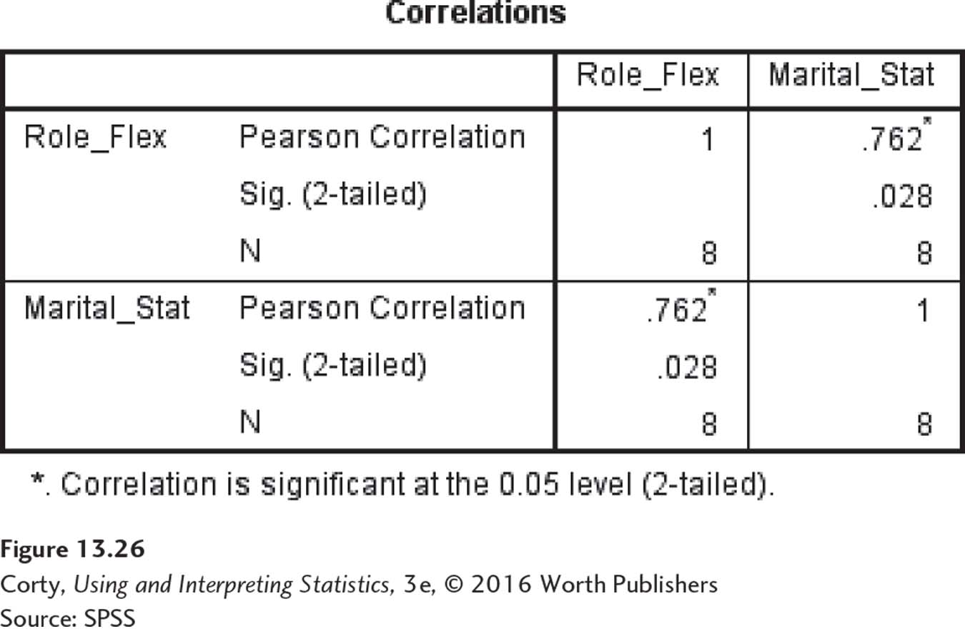
Underneath the value of the correlation is the number .028. This is the significance level for the correlation. If the value is less than or equal to .05, which .028 is, then the results are statistically significant. Want some help deciding if the results are statistically significant? Note the asterisk to the right of .762. Because the option to flag significant correlations was left on, SPSS places an asterisk next to correlations that are significant at the α = .05 level, two-tailed.
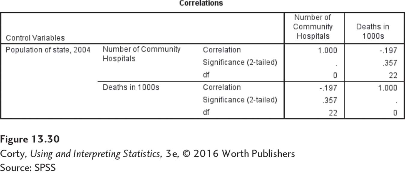
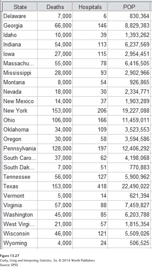
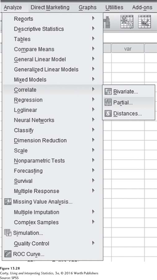
For an example of partial correlation, return to the correlation between number of hospitals and number of deaths when controlling for the population value. We will use a data set with values on these three variables from 25 states, as shown in Figure 13.27. The commands for a partial correlation in SPSS are found under “Analyze,” then “Correlate,” and finally “Partial,” as shown in Figure 13.28.
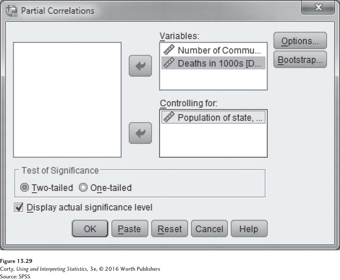
Clicking on “Partial” opens the menu seen in Figure 13.29. The two variables we want to correlate, hospitals and deaths, have been moved into the “Variables” box. The variable we want to control for, “population,” has been moved into the “Controlling for” box. In Figure 13.29, note that the SPSS default options include a two-tailed test and the option to display significant correlations.
The SPSS output is shown in Figure 13.30. SPSS does each partial correlation twice (X with Y and Y with X) and displays the results in what is called a correlation matrix. In the chapter, the correlation between hospitals and deaths controlling for population was –.15. Due to differences in rounding, SPSS reports r = –.197 which is nonsignificant as indicated by the significance value of .357, which exceeds .05.