16.4 Hypothesis Tests II: Relationship Tests
Having covered the selection of descriptive statistics and difference tests, it is time to turn to relationship tests. Relationship tests are meant to examine whether a correlation exists between two variables. Relationship tests are used when there is one sample of cases and each case is measured on two variables in order to see if the variables vary together systematically. For example, one might measure both attractiveness and number of dates in college students to see if the two are associated. The flowchart for selecting the correct relationship test is shown in Figure 16.6.
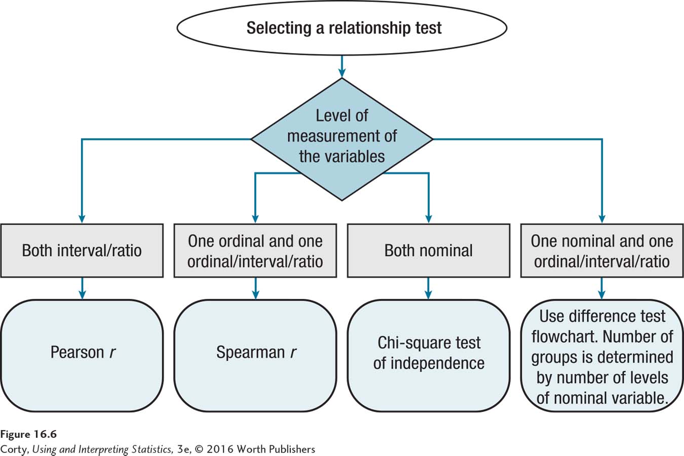
The decision about which relationship test to use in a given situation is determined by the level of measurement for each of the two variables:
If both variables are measured at the interval or ratio level, then the Pearson r is used (see Chapter 13).
If one variable is ordinal and the other is ordinal or interval or ratio, use a Spearman r (see Chapter 15).
If both variables are nominal-level, then the chi-square test of independence is used (see Chapter 15).
When one of the variables is nominal and the other is not, the relationship question can be conceptualized as a difference question. To do so, treat the nominal variable as the explanatory variable and use it to classify cases into groups. Then, the difference test flowchart (Figure 16.5) can be used to determine the appropriate test.
For an example of how to select the correct relationship test, imagine an animal behaviorist who first trained rats to run a maze to find food in a goal box and then measured how many days it took for the behavior to cease (for the rats to stop running to the goal box) once food was no longer being placed in the goal box. She wondered if smarter rats, those who learned the maze more quickly, were also quicker in learning a reward was no longer present. Is there a relationship between the times it takes to learn these two tasks?
This calls for a relationship test. To select the appropriate test, use the flowchart in Figure 16.6. To use that flowchart, the level of measurement must be known for each of the two variables—number of trials to learn the maze and number of days to extinction. Using the flowchart in Figure 16.2, both variables are classified as being at the ratio level. Turning back to the relationship test flowchart, Figure 16.6, when both variables are measured at the interval or ratio level, the Pearson r is the test to use.
Let’s complete one more relationship test example, one in which one variable is nominal and the other isn’t. Imagine a researcher who has a random sample of male college students and a random sample of female college students, and who wonders if there is a relationship between sex (male or female) and GPA. To determine what statistical test should be used, go to the relationship test flowchart, Figure 16.6. Notice that one variable is nominal (sex) and the other variable is interval (GPA). This combination of variables prompts us to exit the relationship test flowchart and move to the difference test flowchart. The relationship question is now phrased, “Is there a difference between male and female students in terms of mean GPA?”
In the difference test flowchart, the nominal-level variable, sex, is treated as the explanatory variable, and the interval/ratio variable, GPA, as the dependent variable. Here are the answers to the choice points in Figure 16.5 for the sex/GPA test decision:
The explanatory variable has two levels, male and female, so two groups are being compared.
Each sample was a random sample from its population, so the two samples are independent.
The dependent variable, GPA, is measured at the interval level.
These choice points lead to the selection of an independent-samples t test as the appropriate test to analyze the data to determine if a relationship exists between sex and mean GPA. A difference test can answer a relationship question.
Worked Example 16.2
A criminologist developed a theory that elementary school teachers can quickly tell which kids are going to be a problem in their classroom. After only two weeks of school, he had asked teachers to make a judgment for each child: whether he or she “would be trouble in the classroom.” A dozen years later, as the same kids are ready to graduate from high school, he tracked down all their records and determined which ones had been arrested, spent time in jail, dropped out of school, and so on. Anyone for whom one of these events had occurred was classified as “having gotten into trouble in life.” What test should the criminologist use to see if an association exists between a prediction made by a first-grade teacher, after only two weeks of observation, and getting into serious trouble over the next 12 years?
This means asking if there is a relationship between the two variables, so the place to start is with the flowchart in Figure 16.6. The first question concerns the level of measurement of the variables. Both variables are nominal. Thus, the appropriate statistical test is the chi-square test of independence.
Practice Problems 16.3
Select the correct statistical test.
16.07 A hair salon owner watches people walk by his shop, notes whether they are male or female, and classifies them as having long hair or short hair. Does a relationship exist between sex and hair length?
16.08 Is there a relationship, for adults, between how many text messages they send per week and how many minutes they talk on their phones?
16.09 An education researcher wants to see if class rank in high school is associated with class rank in college.
Application Demonstration
To see how selecting the correct statistical test works in real life, here are three classic studies in psychology: one that uses descriptive statistics, one that uses difference tests, and one that uses relationship tests.
Obedience to Authority
Perhaps the most famous study in psychology was reported by Stanley Milgram in 1963. Called a “behavioral study in obedience,” Milgram investigated whether normal people would behave in inhumane ways just because they were following orders.
In the study, 40 males, from age 20 to 50, served as participants and were called “teachers.” The teachers were asked to test another participant, called the “learner,” to see how well he had memorized a list of words. For every word the learner got wrong, the teacher was asked to punish him with a shock. And, after delivering a shock, the teacher was to adjust the shock generator to deliver a higher level of shock as the next punishment. The shock generator had 30 levels, ranging from 15 to 450 volts, and the levels were labeled from “Slight Shock” to “Danger: Severe Shock.” At 300 volts, the learner stopped responding—presumably, he was now unconscious or dead from the shocks—and the teacher was instructed to treat no response as a wrong answer, to administer a shock, and to advance to the next question. (By the way, the learner was a confederate of the experimenter, offered incorrect answers according to a script, and received no shocks.)
This is all that there was to Milgram’s experiment. It included no experimental group vs. control group aspect. All he included was an experimental group. Milgram’s question was simple: How many participants would continue to give shocks all the way up to 450 volts? And his answer—a descriptive statistic that 26 of 40 normal men, 65%, were willing to shock a man to death in a psychology experiment simply because a researcher in a lab coat asked them to—shocked a nation. Sometimes the simplest statistic is the most powerful.
Television and Aggression
Leonard Eron was one of the first to study the relationship between children watching violence on TV and behaving aggressively in real life. In 1972, along with some colleagues, he presented data on children followed for 10 years, from 9 to 19 years old.
When the children were 9 years old, the researchers measured the number of violent shows the children liked to watch. At the same time, Eron asked the children to answer questions about their peers. From this, he was able to develop a measure for each child as to how aggressive he or she was, as rated by peers. Similar measures were obtained when the kids were 19 years old.
Eron used Pearson correlation coefficients to analyze the results. Here are the highlights of his findings:
There was a positive, statistically significant correlation of .21 between violent TV watching at age 9 and rating of aggressiveness by peers at age 9.
The correlation between watching violent TV at age 9 and rating of aggressiveness by peers 10 years later was also positive and statistically significant. But, the relationship was stronger one: r = 31.
The correlation between violent TV watching at age 19 and aggression at age 19 was not statistically different from zero.
Taken together, these correlations suggest that early viewing of violent TV is more strongly related to aggression 10 years later than it is to aggression as a child. These relationship tests suggest that there is a critical period in childhood during which images from television may have an impact on personality. Eron’s research has led to thousands of other studies about the effects of violence on television. Simple correlations can make powerful points.
Language and Memory
Elizabeth Loftus, a cognitive psychologist, is one of the people most responsible for eyewitness testimony no longer being held in high esteem. One of her early studies, published with John Palmer in 1974, used difference tests to make this point.
In that study, participants were shown movies of car crashes and asked to estimate how fast the cars were traveling when the crash occurred. Different participants were asked slightly different questions, ranging from how fast the cars were going when they contacted each other to how fast they were going when they smashed into each other. There were five different options: smashed, collided, bumped, hit, and contacted. Loftus’s research question was whether the different words would elicit different estimates of speed.
And, that was what she found. Asked how fast cars were traveling when they “contacted” each other, the mean response was 32 mph. Each word that suggested more speed was associated with an increase of perceived speed by about 2 mph, until cars that “smashed into” each other were going almost 41 mph. The analysis of variance that Loftus used to analyze these results showed that the results were statistically significant. Here’s a difference test that made a difference—it showed that perceptions can be manipulated by a person asking about them.
DIY
Many people have pet theories about the world. A friend of mine in graduate school, many years ago, believed that no matter what she bought at the grocery store, the cost always turned out to be about $15 per bag. I believe that the day after a presidential election, many more supporters of the loser have removed bumper stickers from their cars than have supporters of the winner.
Do you have a pet theory? If not, develop one. What statistical test would you use to answer it?