5.2 Sampling Distributions and the Central Limit Theorem
 StatClips: The Central Limit Theorem Part IVideo on LaunchPad
StatClips: The Central Limit Theorem Part IIVideo on LaunchPad
StatClips: Sampling Distributions Overview and Motivation Part IVideo on LaunchPad
StatClips: Central Limit Theorem Part IIIVideo on LaunchPad
StatClips: Sampling Distributions: Overview and Motivation Part II, Lake Full of Fish ExampleVideo on LaunchPad
Sampling Distributions
The histogram for the percentage of red M&Ms in 500 bags of M&Ms, Figure 5.2, is an example of a sampling distribution. A sampling distribution is generated by (1) taking repeated, random samples of a specified size from a population; (2) calculating some statistic (like a mean or the percentage red M&Ms) for each sample; and (3) making a frequency distribution of those values.
To understand sampling distributions, let’s use an example with a very small population. This example involves a small town in Texas that has a population of only five people (Diekhoff, 1996). Each person is given an IQ test and their five scores can be seen in Figure 5.3. The frequency distribution for these data forms a flat line and does not look like a normal distribution.
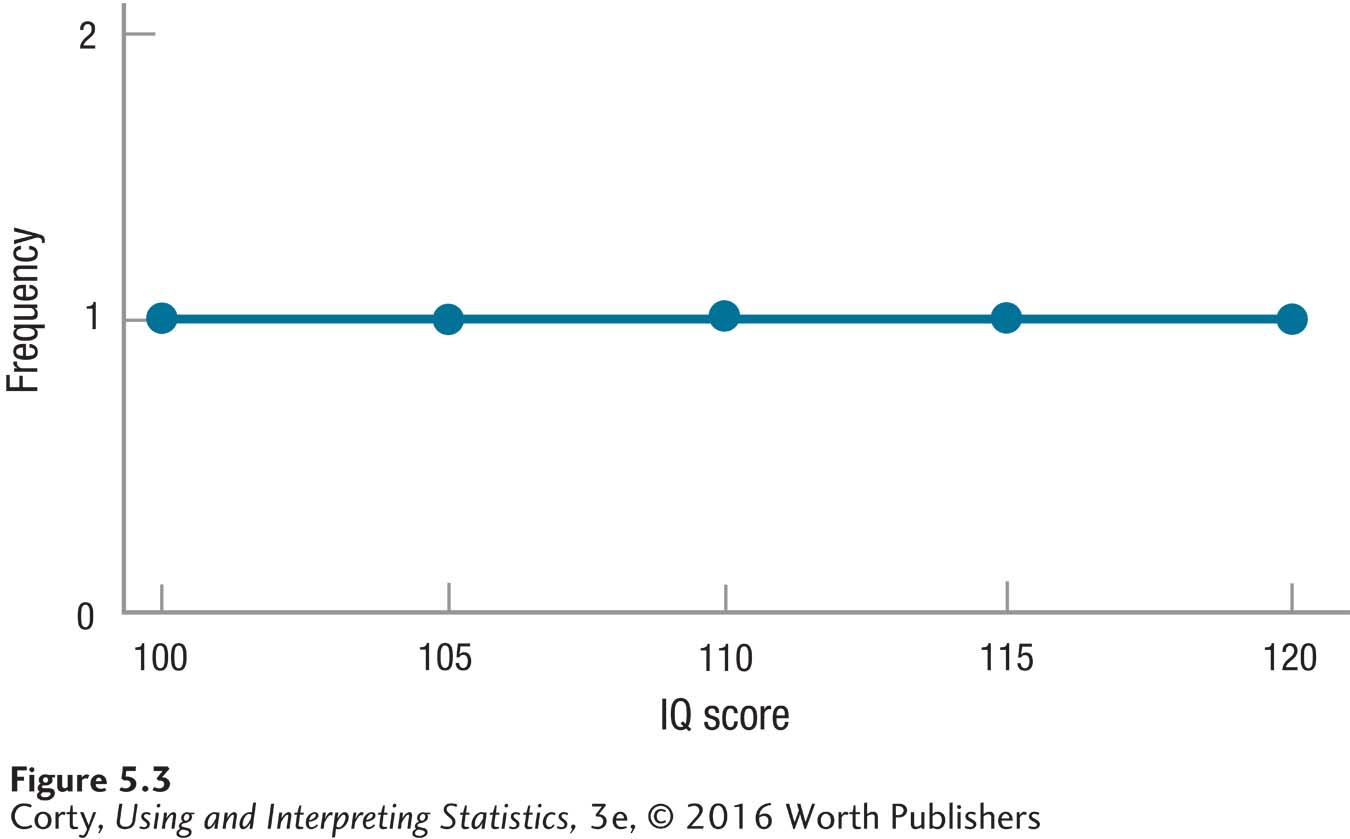
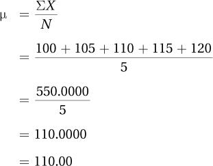
These five people make up the entire population of the town. As there is access to all the cases in the population, this is one of those rare instances where one can calculate a population mean:
To make a sampling distribution of the mean for this population: (1) take repeated, random samples from the population; (2) for each sample, calculate a mean; (3) make a frequency distribution of the sample means. That’s a sampling distribution of the mean.
There are two things to be aware of with regard to sampling distributions:
First, sampling occurs with replacement. This means after a person is selected at random and his or her IQ is recorded, the person is put back into the population, giving him or her a chance to be in the sample again.
Second, the order in which cases are drawn doesn’t matter. A sample with person A drawn first and person B second is the same as person B drawn first and A second.
Our sampling distribution of the mean will have samples of size N = 2. There are 15 possible unique samples of size N = 2 for this Texas town. They are shown in the first panel in Table 5.2.
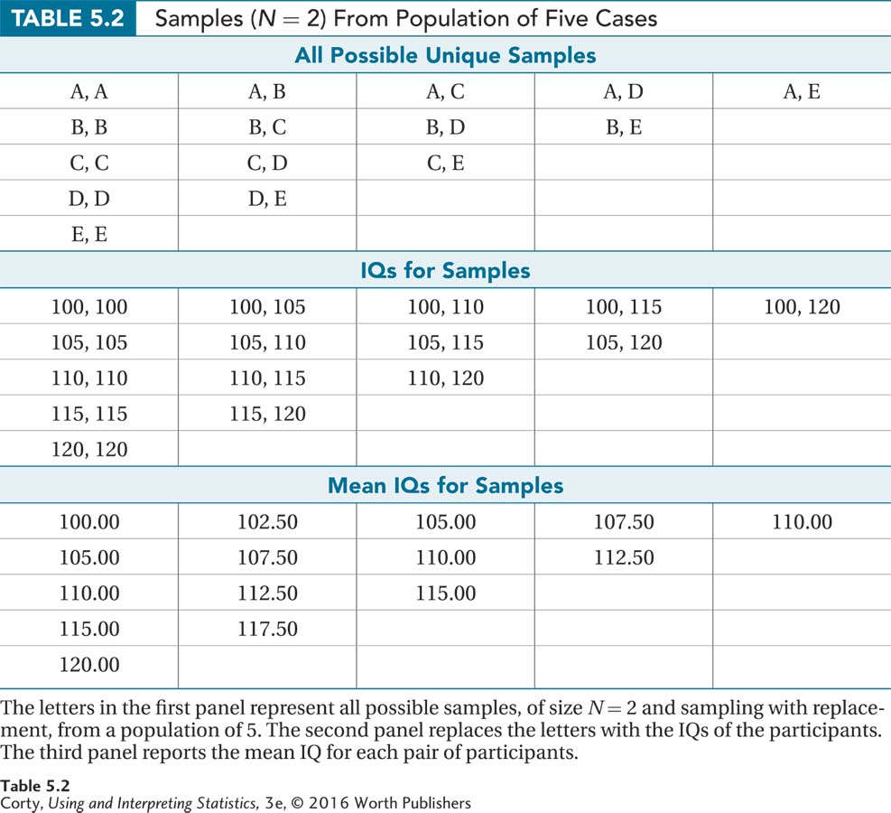
Table 5.2 also shows the pairs of IQ scores for each of the samples (panel 2), as well as the mean IQ score for each sample (panel 3). Note that not all of the sample means are the same. As there is variability in the means, it is possible to calculate a measure of variability (like a standard deviation) for the sampling distribution. Standard error of the mean (abbreviated σM) is the term used for the standard deviation of a sampling distribution of the mean. The standard error of the mean tells how much variability there is from sample mean to sample mean.
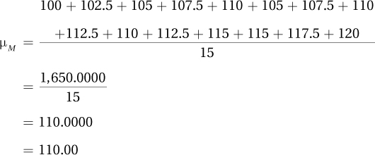
Figure 5.4 shows the sampling distribution for the 15 means from the bottom panel of Table 5.2. The first thing to note is the shape. The population (see Figure 5.3) was flat, but the sampling distribution is starting to assume a normal shape. This normal shape is important because statisticians know how to use z scores to calculate the likelihood of a score falling in a specified segment of the normal distribution.
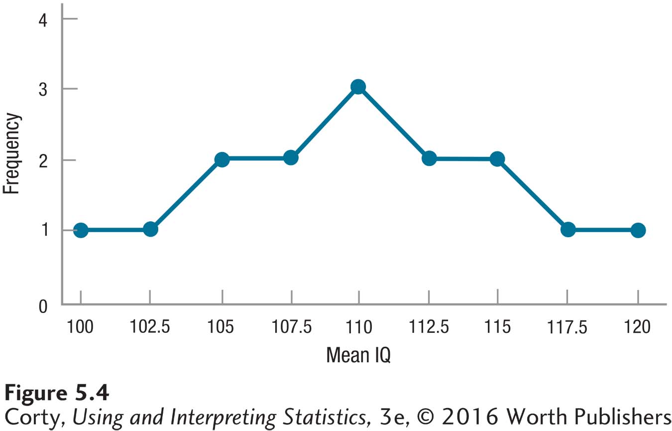
The mean of this sampling distribution is abbreviated as μM because it is a population mean of sample means. Calculating it leads to an interesting observation—the mean of the sampling distribution is the same as the population mean:
The Central Limit Theorem
Having made a number of observations from the sampling distribution for IQ in the small Texas town, it is time to introduce the central limit theorem. The central limit theorem is a description of the shape of a sampling distribution of the mean when the size of the samples is large and every possible sample is obtained.
Imagine someone had put together a sample of 100 Americans and found the mean IQ score for it. What would the sampling distribution of the mean look like for repeated, random samples with N = 100? With more than 300 million people in the United States, it would be impossible to obtain every possible sample with N = 100. That’s where the central limit theorem steps in—it provides a mathematical description of what the sampling distribution would look like if a researcher obtained every possible sample of size N from a population.
Keep in mind that the central limit theorem works when the size of the sample is large. So which number is the one that needs to be large?
Is it the size of the population, which is 5 for the Texas town example?
Is it the size of the repeated, random samples that are drawn from the population? These have N = 2 for the town in Texas.
Is it the number of repeated, random samples that are drawn from the population? This was 15 for the Texas town.
The answer is B: the large number needs to be the number of cases in the sample.
How large is large? An N of 2 is certainly not large. Usually, an N of 30 is considered to be large enough. So, the central limit theorem applies when the size of the samples that make up the sampling distribution is 30 or larger. This means that the researcher with a sample of 100 Americans can use the central limit theorem.
The central limit theorem is important because it says three things:
If N is large, then the sampling distribution of the mean will be normally distributed, no matter what the shape of the population is. (In the small town IQ example, the population was flat, but the sampling distribution was starting to look normal.)
If N is large, then the mean of the sampling distribution is the same as the mean of the population from which the samples were selected. (This was true for our small town example.)
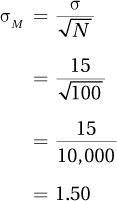
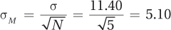
If N is large, then a statistician can compute the standard error of the mean (the standard deviation of the sampling distribution) using Equation 5.1.
Equation 5.1 Formula for Calculating the Standard Error of the Mean

where σM = the standard error of the mean
σ = the standard deviation of the population
N = the number of cases in the sample
Given the sample of 100 Americans who were administered an IQ test that had a standard deviation of 15, the standard error of the mean would be calculated as follows:
When σ Is Not Known
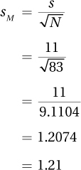
Access to the entire population is rare and it is rare that σ, the population standard deviation, is known. So, how can the standard error of the mean be calculated without σ? In such a situation, one uses the sample standard deviation s, an estimate of the population standard deviation, to calculate an estimated standard error of the mean. The formula for the estimated standard error of the mean, abbreviated sM, is shown in Equation 5.2.
Equation 5.2 Formula for Estimated Standard Error of the Mean

where sM = the estimated standard error of the mean
s = the sample standard deviation (Equation 3.7)
N = the number of cases in the sample
Suppose a nurse practitioner has taken a random sample of 83 American adults, measured their diastolic blood pressure, and calculated s as 11. Using Equation 5.2, he would estimate the standard error of the mean as
A reasonable question to ask right about now is: What is the big deal about the central limit theorem? How is it useful? Thanks to the central limit theorem, a researcher doesn’t need to worry about the shape of the population from which a sample is drawn. As long as the sample size is large enough, the sampling distribution of the mean will be normally distributed even if the population isn’t. This is handy, because the percentages of cases that fall in different parts of the normal distribution is known.
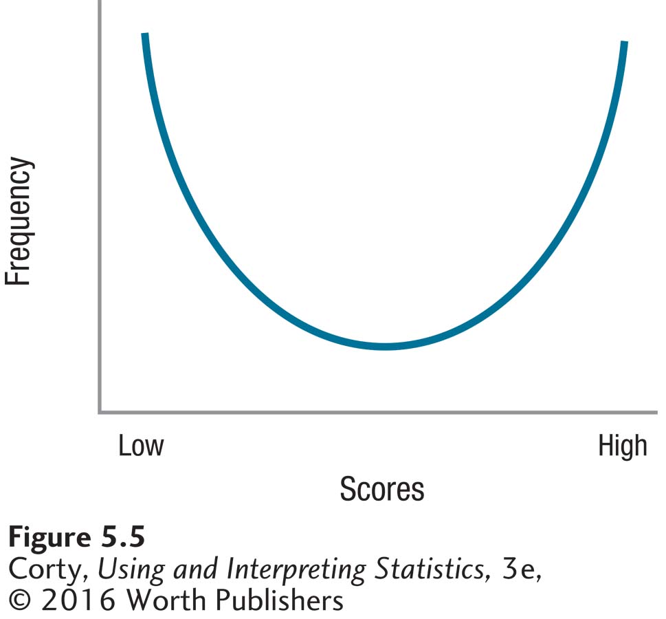
Look at the shape of the population displayed in Figure 5.5. It is far from normal. Yet, if one were to take repeated random samples from this population, calculate a mean for each sample, and make a sampling distribution of the means, then that sampling distribution would look normal as long as the sample sizes were large. This is advantageous because when hypothesis testing is introduced in the next chapter, the hypotheses being tested turn out to be about sampling distributions. If the shape of a sampling distribution is normal, then it is possible to make predictions about how often a particular value will occur.
Another benefit of the central limit theorem is that it allows us to calculate the standard error of the mean from a single sample. What’s important about the standard error of the mean? A smaller standard error of the mean indicates that the means in a sampling distribution are packed more closely together. This tells us that there is less sampling error, that the sample means tend to be closer to the population mean. If the standard error of the mean is small, then a sample mean is probably a more accurate reflection of the population mean because it likely falls close to the population mean.
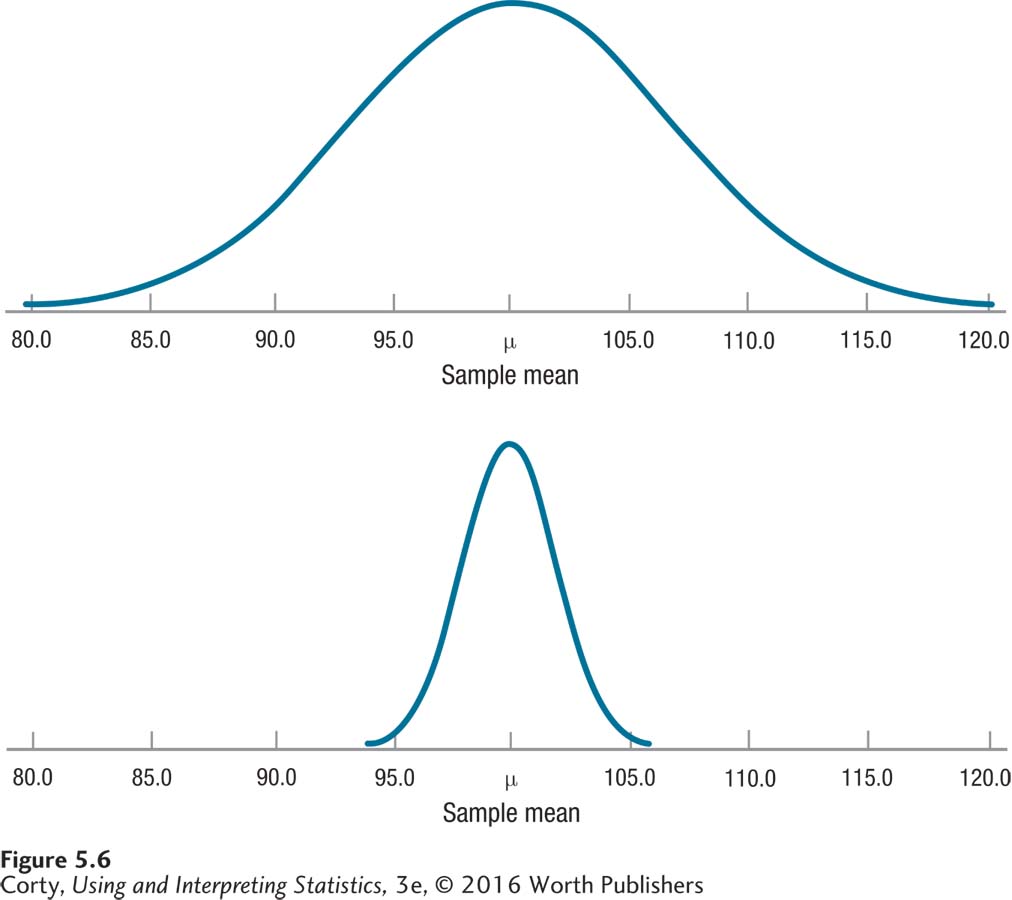
In a sense, a sampling distribution is a representation of sampling error. Figure 5.6 shows this graphically. Note how the distribution with a larger sample size has less variability and is packed more tightly around the population value. It has less sampling error.
A Common Question
Q Are sampling distributions only for means?
A No, a sampling distribution can be constructed for any statistic. There could be a sampling distribution of standard deviations or of medians. In future chapters, sampling distributions of statistics called t, F, and r will be encountered.
Worked Example 5.2
Sampling distribution generators (available online) draw thousands of samples at a time and form a sampling distribution in a matter of seconds right on the computer screen. A researcher can change parameters—like the shape of the parent population, the size of the samples, or the number of samples—and see the impact on the shape of the sampling distribution. Nothing beats playing with a sampling distribution generator for gaining a deeper understanding of the central limit theorem. Google “Rice Virtual Lab in Statistics,” click on “Simulations/Demonstrations,” and play with the “sampling distribution simulation.” For those who prefer a guided tour to a self-guided one, read on.
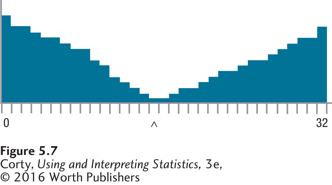
Figure 5.7 uses the Rice simulation to show a population constructed not to be normal. In this population, scores range from 0 to 32, μ = 15.00, σ = 11.40, and the midpoint does not have the greatest frequency.
The Rice simulator allows one to control how large the samples are and how many samples one wishes to take from the population. Figure 5.8 illustrates one random sample of size N = 5 from the population. The left panel in Figure 5.8 shows the five cases that were randomly selected and the right panel the mean of these five cases, the first sample. Note that the five cases are scattered about and that the sample mean (M = 16.00) is in the ballpark of the population mean (μ = 15.00), but is not an exact match.
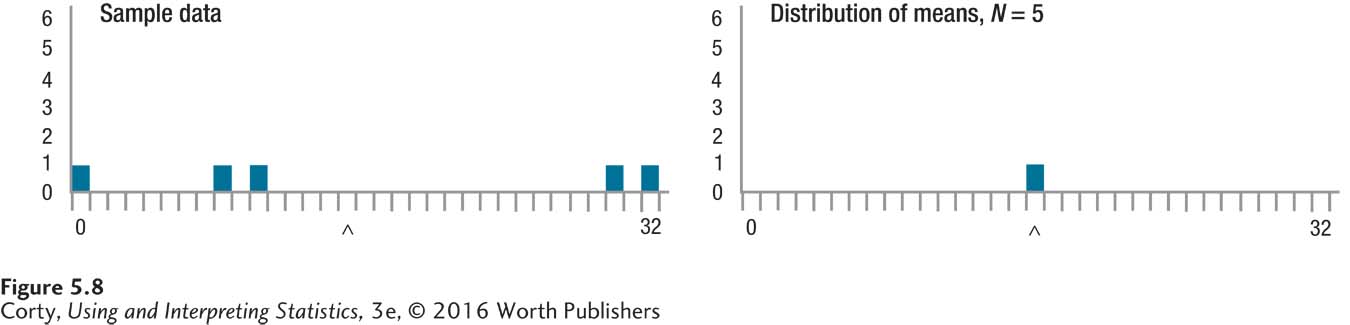
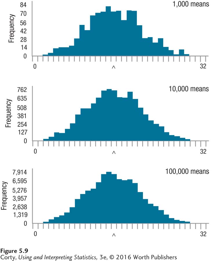
Figure 5.9 shows the sampling distribution after 1,000 random samples were drawn, after 10,000 random samples were drawn, and after 100,000 random samples were drawn. There are several things to note:
All three of the sampling distributions have shapes that are similar to those of a normal distribution, despite the fact that the parent population is distinctly non-normal. This is predicted by the central limit theorem.
As the number of samples increases, the distribution becomes smoother and more symmetrical. But, even with 100,000 samples, the sampling distribution is not perfectly normal.
Page 158The central limit theorem states that the mean of a sampling distribution is the mean of the population. Here, the population mean is 15.00, and the mean of the sampling distribution gets closer to the population mean as the number of samples in the distribution grows larger. With 1,000 samples M = 15.15, with 10,000 M = 15.02, and with 100,000 it is 15.00.
Notice the wide range of the means in the sampling distribution—some are at each end of the distribution. With a small sample size, like N = 5, one will occasionally draw a sample that is not representative of the population and that has a mean far away from the population mean. This is due entirely to the random nature of sampling error.
The central limit theorem states that the standard error of the mean, which is the standard deviation of the sampling distribution, can be calculated from the population standard deviation and the size of the samples:
 . This is quite accurate—the standard deviations of the three sampling distributions are 5.06, 5.19, and 5.12.
When the size of the random samples increases from N = 5 to N = 25, some things change about the shape of the sampling distribution, as can be seen in Figure 5.10. It, like Figure 5.9, shows sampling distributions with 1,000, 10,000, and 100,000 samples. But, unlike Figure 5.9, the changes in the sampling distribution as the numbers of samples increase are more subtle. All three sampling distributions have a normal shape, though as the number of samples increases from 1,000 to 10,000, there is a noticeable increase in symmetry.
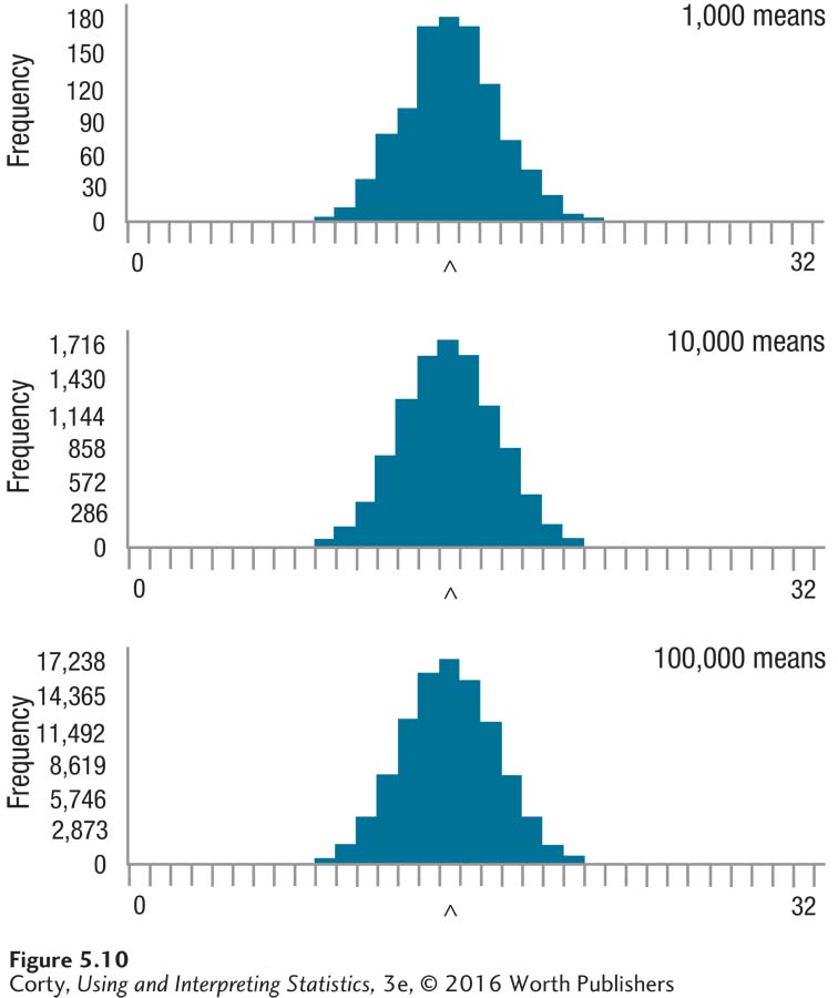
The most noticeable difference between the sampling distributions based on smaller samples, seen in Figure 5.9, and those based on larger samples, seen in Figure 5.10, lies in the range of means. In Figure 5.9, the means ranged from 2 to 29, while in Figure 5.10, they range from 9 to 22. There is less variability in the sampling distribution based on the larger samples.
This decreased variability is mirrored in the standard deviations. (Remember, the standard deviation of the sampling distribution is the standard error of measurement. When 100,000 samples of size N = 5 are taken, the standard deviation of the sampling distribution was 5.12. When the same number of samples is taken, but the size of each sample is 25, not 5, the standard deviation of the sampling distribution falls to 2.28. This is exactly what is predicted for the standard error of the mean by the central limit theorem:
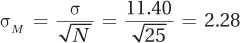
As was mentioned above, when the standard error of the mean is smaller, the means are packed more tightly together and less sampling error exists. A larger sample size means that there is less sampling error and that the sample is more likely to provide a better representation of the population.
Practice Problems 5.2
Review Your Knowledge
5.06 What is a sampling distribution?
5.07 What are three facts derived from the central limit theorem?
Apply Your Knowledge
5.08 There’s a small town in Ohio that has a population of 6 and each person has his or her blood pressure measured. The people are labeled as A, B, C, D, E, and F. If one were to draw repeated, random samples of size N = 2 to make a sampling distribution of the mean, how many unique samples are there?
5.09 Researcher X takes repeated, random samples of size N = 10 from a population, calculates a mean for each sample, and constructs a sampling distribution of the mean. Researcher Y takes repeated, random samples of size N = 100 from the same population, calculates a mean for each sample, and constructs a sampling distribution of the mean. What can one conclude about the shapes of the two sampling distributions?
5.10 If σ = 12 and N = 78, what is σM?