6.3 Type I Error, Type II Error, Beta, and Power
Imagine a study in which a clinical psychologist, Dr. Cipriani, is investigating if a new treatment for depression works. One way that her study would be successful is if the treatment were an effective one and the data she collected showed that. But, her study would also be successful if the treatment did not help depression and her data showed that outcome.
Those are “good” outcomes; there are also two “bad” outcomes. Suppose the treatment really is an effective one, but her sample does not show this. As a result of such an outcome, this effective treatment for depression might never be “discovered.” Another bad outcome would occur if the treatment were in reality an ineffective one, but for some odd reason it worked on her subjects. As a result, this ineffective treatment would be offered to people who are depressed and they would not get better.
Table 6.5 shows the four possible outcomes for hypothesis tests. The two columns represent the reality in the population. The column on the left says the null hypothesis is really true. In Dr. Cipriani’s terminology, this means treatment has no impact. The column on the right says the treatment does make a difference; the null hypothesis is not true. The two rows represent the conclusions based on the sample. The top row says that the results fell in the common zone, meaning that the researcher will fail to reject the null hypothesis. (Dr. Cipriani will conclude that her new treatment does not work.) The bottom row says that the results fell in the rare zone, so the researcher will reject the null hypothesis. (Dr. Cipriani will conclude that her treatment works.)
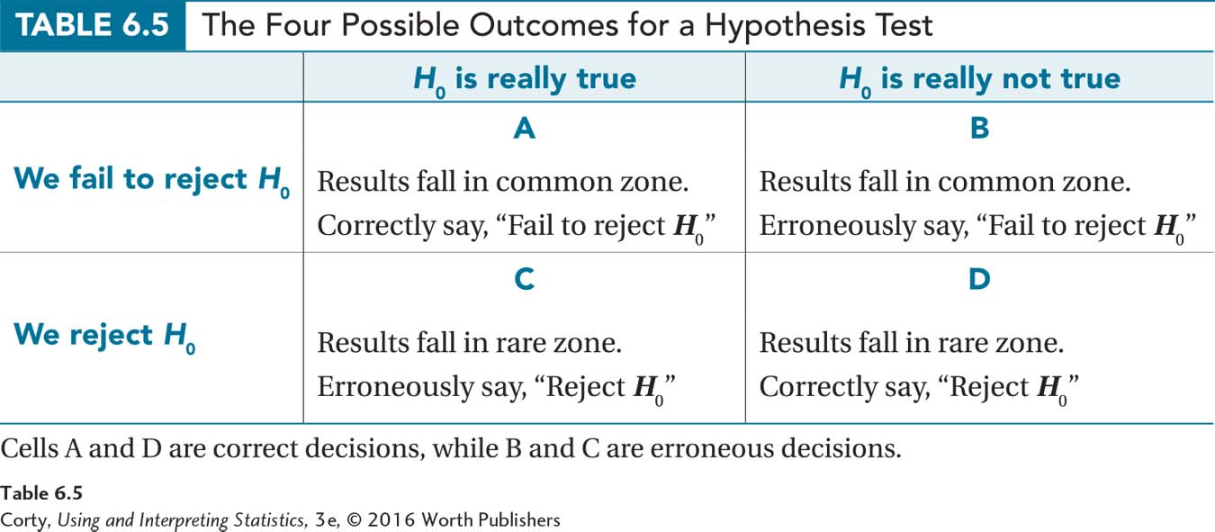
The two scenarios in which a study would be considered a success are Outcome A and Outcome D. In Outcome A, in the terminology of hypothesis testing, a researcher correctly fails to reject the null hypothesis. For Dr. Cipriani, this outcome means that treatment is ineffective and the evidence of her sample supports this. In Outcome D, the null hypothesis is correctly rejected. For Dr. Cipriani, the treatment does work and she finds evidence that it does.
The two other outcomes, Outcome B and Outcome C, are bad outcomes for a hypothesis test because the conclusions would be wrong. In Outcome B, the researcher fails to reject the null hypothesis when it should be rejected. If this happened to Dr. Cipriani, she would say that there is insufficient evidence to indicate the treatment works and she would be wrong as the treatment really does work. In Outcome C, a researcher erroneously rejects the null hypothesis. If Dr. Cipriani concluded that treatment works, but it really doesn’t, she would have erroneously rejected the null hypothesis.
A problem with hypothesis testing is that because the decision relies on probability, a researcher can’t be sure if the conclusion about the null hypothesis is right (Outcomes A or D) or wrong (Outcomes B or C). Luckily, a researcher can calculate the probability that the conclusion is in error and know how probable it is that the conclusion is true. With hypothesis testing, one can’t be sure the conclusion is true, but one can have a known degree of certainty.
Type I Error
Let’s start the exploration of errors in hypothesis testing with Outcome C, a wrong decision. When a researcher rejects the null hypothesis and shouldn’t have, this is called a Type I error. In the depression treatment example, a Type I error occurs if Dr. Cipriani concludes that the treatment makes a difference when it really doesn’t. If that happened, psychologists would end up prescribing a treatment that doesn’t help.
Routinely, researchers decide they are willing to make a Type I error 5% of the time.
Routinely, researchers decide they are willing to make a Type I error 5% of the time. Five percent is an arbitrarily chosen value, but over the years it has become the standard value. One doesn’t need to use 5%. If the consequences of making a Type I error seem particularly costly, one might be willing only to risk a 1% chance of this mistake. For example, imagine using a test to select technicians for a nuclear power plant. The potential catastrophe if the wrong person is hired is so great that the cut-off score on the test should be very high. On the other hand, if making a Type I error doesn’t seem consequential—for example, if one is hiring people for a task that doesn’t have serious consequences for failure—then one might be willing to live with a greater chance of this error.
The likelihood of Type I error is determined by setting the alpha level. As alpha gets larger, so does the rare zone. A larger rare zone makes it easier to reject the null hypothesis. Figure 6.6 shows the common and rare zones for a single-sample z test for three common alpha levels (α = .10, α = .05, and α = .01). Note that as alpha decreases, so does the size of the rare zone, making it more difficult to reject the null hypothesis.
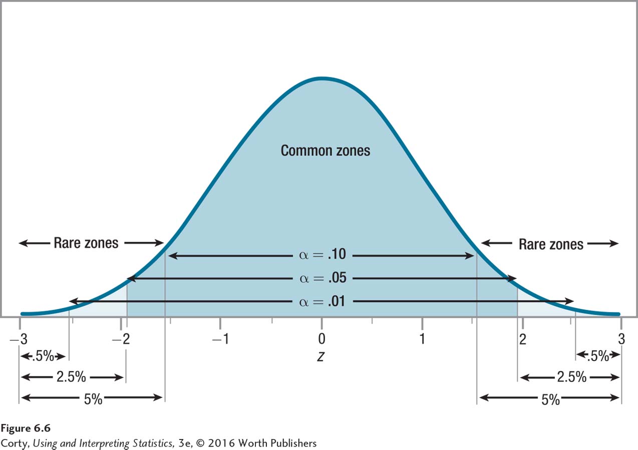
Setting alpha at .05 gives a modest chance of Type I error and a reasonable chance of being able to reject the null hypothesis.
Making errors is never a good idea, so why isn’t alpha always set at .01 or even lower? The reason is simple. When alpha is set low, it is more difficult to reject the null hypothesis because the rare zone is smaller. Rejecting the null hypothesis is almost always the goal of a research study, so researchers would be working against themselves if they made it too hard to reject the null hypothesis. When setting an alpha level, a researcher tries to balance two competing objectives: (1) avoiding Type I error and (2) being able to reject the null hypothesis. The more likely one is to avoid Type I error, the less likely one is to reject the null hypothesis. The solution is a compromise. Setting alpha at .05 gives a modest chance of Type I error and a reasonable chance of being able to reject the null hypothesis.
Type II Error and Beta
There’s another type of error possible, Type II error. This is Outcome B in Table 6.5. A Type II error occurs when the null hypothesis should be rejected, but it isn’t. If Dr. Cipriani’s new treatment for depression really was effective, but she didn’t find evidence that it was effective, that would be a Type II error.
The probability of making a Type II error is known as beta, abbreviated with the lowercase Greek letter β. The consequences of making a Type II error can be as serious as the consequences of making a Type I error. But, when statisticians attend to beta, they commonly set it at .20. This gives a 20% chance for this error, not a 5% chance as is usually set for alpha.
A researcher only needs to worry about beta when failing to reject the null hypothesis. Let’s use the psychic blood pressure example from Worked Example 6.1—where the null hypothesis wasn’t rejected—to examine how Type II error may occur.
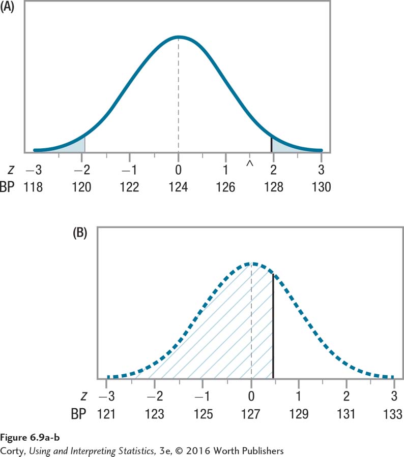
In that study, Dr. Levine studied a sample of 81 people whom a psychic believed had abnormal blood pressure. Their mean blood pressure was 127. The population mean was 124, with σ = 18. Dr. Levine tested the null hypothesis (H0: μ = 124) vs. the alternative hypothesis (H1: μ ≠ 124) using a two-tailed single-sample z test with σ = .05. The critical value of z was ±1.96. After calculating σM = 2.00, he calculated z = 1.50. As z fell in the common zone, he failed to reject the null hypothesis. There was insufficient evidence to say that the psychic could discern people with abnormal blood pressure.
The null hypothesis was tested by assuming it was true and building a sampling distribution of the mean centered around μ = 124. In Figure 6.7, note these four things about the sampling distribution:
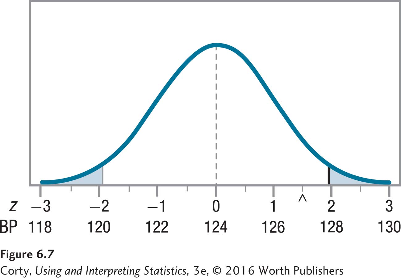
The midpoint—the vertical line in the middle—is marked on the X-axis both with a blood pressure of 124 and a z score of 0.
The other blood pressures marked on the X-axis are two points apart because σM = 2. The X-axis is also marked at these spots with z scores from –3 to 3.
The rare zone, the area less than or equal to a z value of –1.96 and greater than or equal to a z value of 1.96, is shaded. If a result falls in the rare zone, the null hypothesis is rejected.
A caret, ^, marks the spot where the sample mean, 127, falls. This is equivalent to a z score of 1.50 and falls in the common zone. The null hypothesis is not rejected.
Now, imagine that the null hypothesis is not true. Imagine that the population mean is 127 instead of 124. Why pick 127? Because that was the sample mean and is the only objective evidence that we have for what the population mean might be for people the psychic says have high blood pressure.
With this in mind, look at Figure 6.8. The top panel (A) is a repeat of the sampling distribution shown in Figure 6.7, the distribution centered around the mean of 124, the mean hypothesized by the null hypothesis. The bottom panel (B), the dotted line distribution, is new. This is what the sampling distribution would look like if μ = 127. Note these four characteristics about the sampling distribution in the bottom panel:
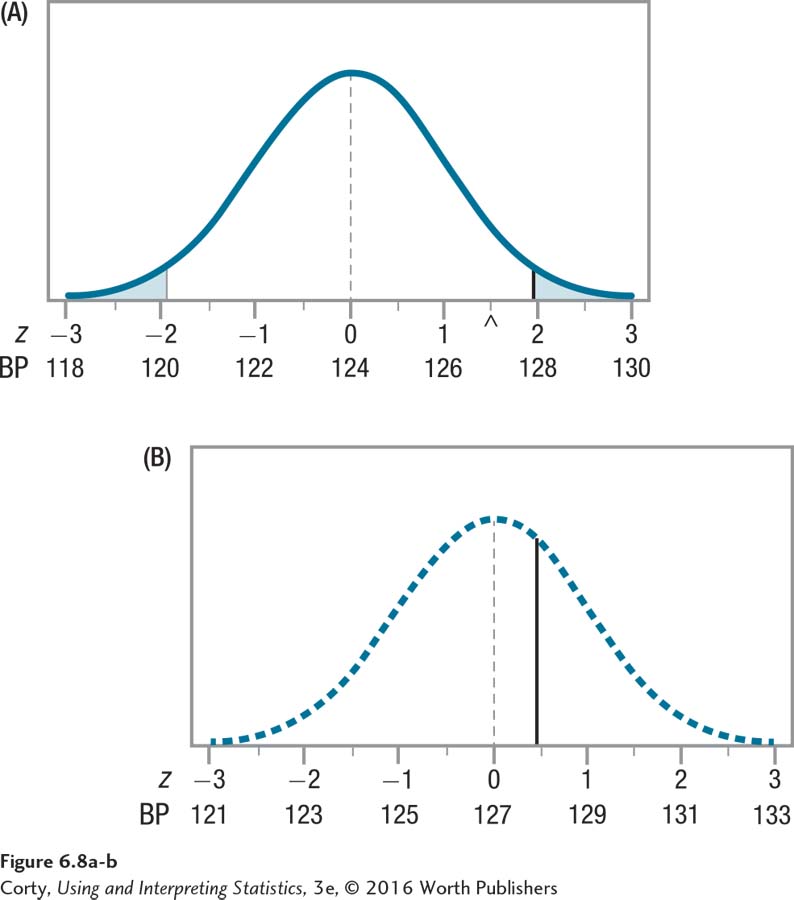
The dotted line sampling distribution has exactly the same shape as the one in the top panel; it is just shifted to the right so that the midpoint, represented by a dotted vertical line, occurs at a blood pressure of 127.
This midpoint, 127, is right under the spot marked by a caret in the top panel. That caret represents where the sample mean, 127, fell.
The other points on the X-axis are marked off by blood pressure scores ranging from 121 to 133, and z scores ranging from –3 to 3.
There is a solid vertical line in the lower panel of Figure 6.8. The vertical line is drawn at the same point as the z score of 1.96 was in the top panel. This vertical line marks the point that was one of the critical values of z in the top panel. In the top panel, scores that fell to the left of this line fell in the common zone and scores that fell on or to the right of the line fell in the rare zone.
Figure 6.9 takes Figure 6.8 and hatches in the area to the left of the vertical line with /// in the bottom panel (B). This area, which is more than 50% of the area under the curve, indicates the likelihood of a Type II error. How so? Well, if μ were really 127, then the null hypothesis that the population mean is 124 should be rejected! However, looking at the top panel (A) to make this decision, a researcher wouldn’t reject the null hypothesis after obtaining a mean that falls in the area hatched like ///. (Remember, the sample means will be spread around the population mean of 127 because of sampling error.) Whenever a sample mean falls in this hatched-in area, a Type II error is committed and a researcher fails to reject a null hypothesis that should be rejected.
Under these circumstances, the researcher would commit a Type II error fairly frequently if the population mean were really 127, but the null hypothesis claimed it was 124. The researcher would commit a Type II error less frequently if the population mean were greater than 127. Right now, the difference between the null hypothesis value (124) and the value that may be the population value (127) is fairly small, only 3 points. This suggests that if the psychic can read blood pressure, he has only a small ability to do so. If the effect were larger, say, the dotted line distribution shifted to a midpoint of 130, the size of the effect, the psychic’s ability to read blood pressure, would be larger. The bottom panel (C) of Figure 6.10 shows the sampling distribution made with a dashed line. This is the sampling distribution that would exist if the population mean were 130. Notice how much smaller the hatched-in error area is in this sampling distribution, indicating a much smaller probability of Type II error.
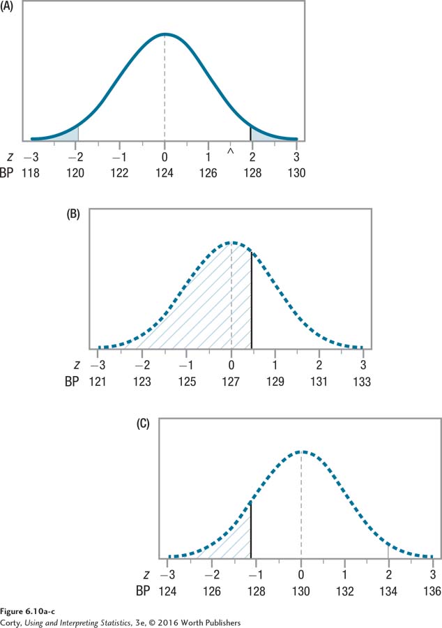
The point is this: the probability of Type II error depends on the size of the effect, the difference between what the null hypothesis says is the population parameter and what the population parameter really is. When the difference between these values is small, the probability of a Type II error is large. Type II error can still occur when the effect size is large, but it is less likely.
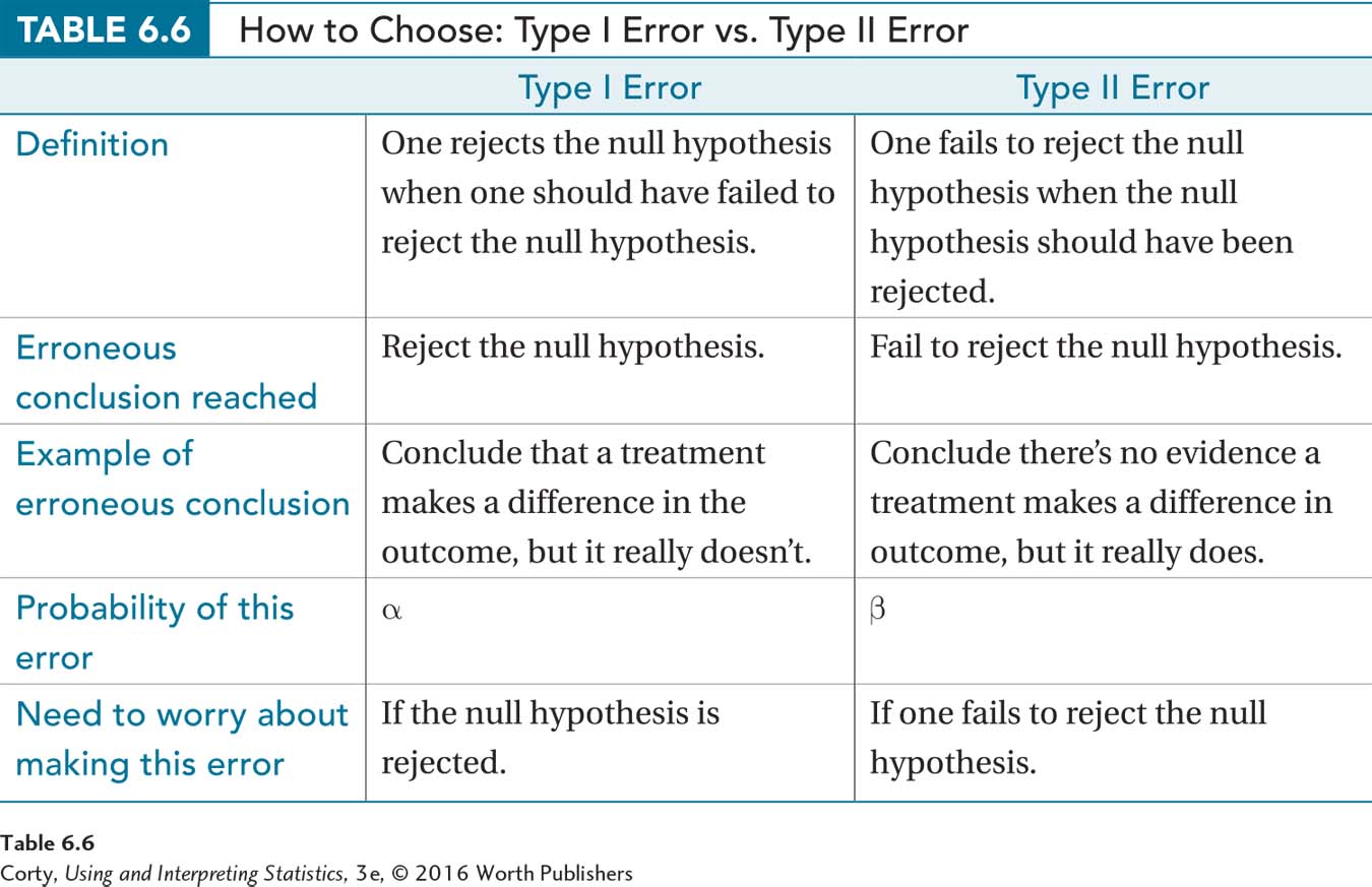
When one is starting out in statistics, it is hard to remember the differences between Type I error and Type II error. Table 6.6 summarizes the differences between the two.
Power
There’s one more concept to introduce before this chapter draws to a close and that is power. Power refers to the probability of rejecting the null hypothesis when the null hypothesis should be rejected. Because the goal of most studies is to reject the null hypothesis and be forced to accept the alternative hypothesis (which is what the researcher really believes is true), researchers want power to be as high as possible.
The area that is hatched \\\ in the bottom panel (C) in Figure 6.11 demonstrates the power of the single-sample z test in Dr. Levine’s psychic blood pressure study. If the population mean is really 127, whenever a sample mean falls in this hatched-in area, the researcher will reject the null hypothesis. Why? Because a population mean in this hatched-in area falls in the shaded-in rare zone shown in the top panel (A).
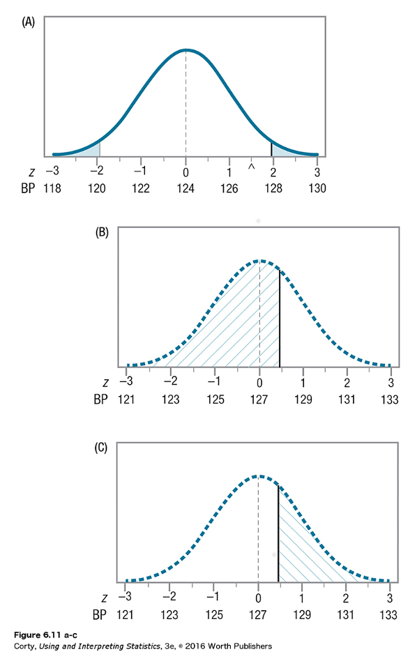
Look at the area hatched in /// in the middle panel (B) of Figure 6.11 and the area hatched in \\\ in the bottom panel (C) of Figure 6.11. The hatched-in area in the middle panel represents beta, the probability of Type II error, while the hatched-in area in the bottom panel represents power. Together, these two hatched-in areas shade in the entire dotted-line curve. This shows that beta and power are flip sides of the same coin. When the null hypothesis should be rejected, beta plus power equals 100% of the area under the dotted-line curve.
Statisticians refer to beta and power using probabilities, not percentages. They would say: β + power = 1.00. If either beta or power is known, the other can be figured out. If beta is set at .20, then power is .80. If power is .95, then beta is .05.
Type I error and Type II error are errors of the conclusion, not errors of the facts on which conclusions are based.
There’s more to be learned about Type I and Type II errors, beta, and power in later chapters. For now, here’s a final point. If a Type I error or a Type II error occurs, this doesn’t mean the results of the study are wrong. After all, the sample mean is the mean that was found for the sample. What a Type I or Type II error means is that the conclusion drawn from the sample mean about the population mean is wrong. Type I error and Type II error are errors of the conclusion, not errors of the facts on which conclusions are based.
Practice Problems 6.3
Review Your Knowledge
6.07 When does Type II error occur?
6.08 What is power?
Apply Your Knowledge
6.09 What is a correct conclusion in hypothesis testing?
6.10 What is an incorrect conclusion in hypothesis testing?
Application Demonstration
To see hypothesis testing in action, let’s leave numbers behind and turn to a simplified version of one way the sex of a baby is identified before it is born. Around the fifth month of pregnancy, an ultrasound can be used to identify whether a fetus is a boy or a girl. The test relies on hypothesis testing to decide “boy” or “girl,” and it is not 100% accurate. Both Type I errors and Type II errors are made. Here’s how it works.
The null hypothesis, which is set up to be rejected, says that the fetus is a girl. Null hypotheses state a negative, and the negative statement here is that the fetus has no penis. Together, the null hypothesis and the alternative hypothesis have to be all-inclusive and mutually exclusive, so the alternative hypothesis is that the fetus has a penis.
The sonographer, then, starts with the hypothesis that the fetus is a girl. If the sonographer sees a penis, the null hypothesis is rejected and the alternative hypothesis is accepted, that the fetus is a boy.
Of course, mistakes are made. Suppose the fetus is a girl and a bit of her umbilical cord is artfully arranged so that it masquerades as a penis. The sonographer would say “Boy” and be wrong. This is a Type I error, where the null hypothesis is wrongly rejected.
A Type II error can be made as well. Suppose the fetus is a shy boy who arranges his legs or hands to block the view. The sonographer doesn’t get a clear view of the area, says “Girl,” and would be wrong. This is a Type II error, wrongly failing to reject the null hypothesis.
However, in this case, a smart sonographer doesn’t say “Girl.” Instead, the sonographer, failing to see male genitalia, indicates that there’s not enough evidence to conclude the fetus is a boy. That is, there’s not enough evidence to reject the hypothesis that it’s a girl. Absence of evidence is not evidence of absence.
DIY
Grab a handful of coins, say, 25, and let’s investigate Type I error. Type I error occurs when one erroneously rejects the null hypothesis. In this exercise, the null hypothesis is going to be that a coin is a fair coin. This means that each coin has a heads and a tails, and there is a 50-50 chance on each toss that a heads will turn up.
For each coin in your handful, you will determine if it is a fair coin by tossing it, by observing its behavior. Imagine you toss the coin once and it turns out to be heads. Does that give you any information whether it is a fair coin or not? No, it doesn’t. A fair coin could certainly turn up heads on the first toss. So, you toss it again and again it turns up heads. Could a fair coin turn up heads 2 times in a row? Yes. There are four outcomes (HH, HT, TH, and TT), one of which is two heads, so two heads in a row should happen 25% of the time. How about three heads in a row? That will happen 12.5% of the time with a fair coin. Four heads? 6.25% of the time. Finally, if there are five heads in a row, we will step over the 5% rule. Five heads in a row, or five tails in a row, will happen only 3.125% of the time with a fair coin. It could happen, but it is a rare event, and when a rare event occurs—one that is unlikely to occur if the null hypothesis is true—we reject the null hypothesis.
So, here’s what you do. Test one coin at a time from your handful. Toss each coin 5 times in a row. If the result is a mixture of heads and tails, which is what you’d expect if the test were fair, there is not sufficient evidence to reject the null hypothesis. But, if it turns up five heads in a row or five tails in a row, you have to reject the null hypothesis and conclude the coin is not fair. If that happens to you, then pick up the coin and examine it. Does it have a heads and a tails? Toss it 5 more times. Did it turn up five heads or five tails again? This time, it probably behaved more like a fair coin.
There are two lessons here. First, occasionally, about 3% of the time, a fair coin will turn up heads 5 times in a row. If that happens, by the rules of hypothesis testing, we would declare the coin unfair. That conclusion would be wrong; it would be a Type I error. If you stopped there, if you did not replicate the experiment, you’d never know that you made a mistake. And that is a danger of hypothesis testing—your conclusion can be wrong and you don’t know it. So here’s the second lesson: replicate. When the same results occur 2 times in a row, you have a lot more faith in them.