External Costs, External Benefits, and Efficiency
Externalities are external costs or external benefits, that is, costs or benefits, respectively, that fall on bystanders.
This chapter is about products, like antibiotics, for which some of the costs or benefits of the product fall on bystanders. These costs or benefits are called external costs or external benefits or, for short, externalities. (External costs are sometimes also called negative externalities, and external benefits are sometimes also called positive externalities.) When externalities are significant, markets work less well and government action can increase social surplus.
Social surplus is consumer surplus plus producer surplus plus everyone else’s surplus.
In Chapter 4, we showed that a market equilibrium maximizes consumer plus producer surplus (the gains from trade). But maximizing consumer plus producer surplus isn’t so great if bystanders are harmed in the process. Everyone counts, not just the consumers and producers of a particular product. So, when we evaluate how well a market with externalities is working, we want to look at social surplus, namely consumer surplus plus producer surplus plus everyone else’s surplus.
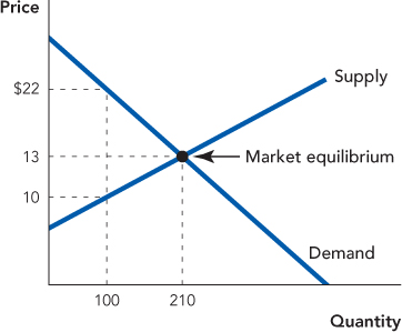
To show why a market with externalities does not maximize social surplus, it’s useful to briefly review why a market equilibrium does maximize consumer plus producer surplus (see also Chapter 4). The key is to remember that you can read the value of the nth unit of a good from the height of the demand curve and the cost of the nth unit of a good from the height of the supply curve. For example, imagine that buyers and sellers are currently exchanging 99 units of a good. What is the value to buyers and the costs to sellers of one additional unit, the 100th unit? In Figure 10.1, you can read the value to buyers from the height of the demand curve at the 100th unit, namely $22. You can read the cost to sellers from the height of the supply curve at the 100th unit, namely $10. Since the value of the 100th unit exceeds the additional cost of the 100th unit, there is an incentive to trade, namely an opportunity to increase consumer and producer surplus. Following this logic, trade is mutually profitable up until the 210th unit is sold. The value to buyers of the 210th unit is $13 and the cost to sellers of producing that additional unit is $13 so at this point there are no further incentives to trade. If any fewer units were traded, gains from trade would be left on the table. If any more units were traded, the cost of those units would exceed their value. Thus, gains from trade are maximized at the market equilibrium of 210 units.
FIGURE 10.1

The efficient equilibrium is the price and quantity that maximizes social surplus.
Let’s call the price and quantity that maximize social surplus the efficient equilibrium. If there are no significant externalities, the market equilibrium is also the efficient equilibrium (because if there are no significant external costs or benefits, maximizing producer plus consumer surplus is the same as maximizing everyone’s surplus). But if there are significant externalities, the market equilibrium is no longer the efficient equilibrium, as we will now show.
External Costs
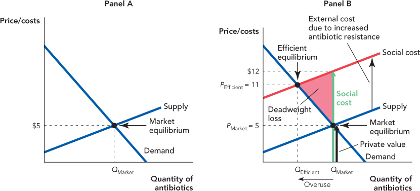
The left panel of Figure 10.2 shows the market equilibrium for antibiotics. As usual, the market equilibrium maximizes consumer plus producer surplus. But now the use of antibiotics creates an external cost, a cost to people who are neither buying nor selling antibiotics. At the market equilibrium, the price of a round of antibiotics—such as your doctor would prescribe to cure an infection—is $5 and we will assume that the external cost of antibiotic use is $7, a number that is consistent with a recent study of the matter.1 The private cost plus the external cost is the social cost of antibiotic use.
In the right panel of Figure 10.2, we add the external cost to the supply curve to show the social cost curve. The social cost curve takes into account all of the costs of antibiotic use so it’s the social cost curve that we use to figure out the efficient quantity, the quantity that maximizes social surplus. The efficient quantity QEfficient is found where the demand curve intersects the social cost curve.
FIGURE 10.2

Panel A: The market equilibrium is found, as usual, where the supply and demand curves intersect. The market equilibrium maximizes consumer plus producer surplus.
Panel B: We add external costs to the supply curve to find the social cost curve. Notice that the social cost of the QMarket unit exceeds the private value of this unit. The efficient equilibrium is found where the social cost and demand curves intersect. QEfficient is less than QMarket so the market overproduces goods with significant external costs.
The efficient quantity is the quantity that maximizes social surplus.
To see exactly why the market equilibrium is not efficient, let’s consider the value to buyers and the social costs of the QMarket unit of the good. The height of the demand curve at the QMarket unit (the black arrow labeled “Private value”) tells us that this unit has a private value of $5. The height of the social cost curve at QMarket (the green arrow labeled “Social cost”) tells us that this unit has a social cost of $12. Thus, producing this unit creates a social loss or deadweight loss of $7. Following this logic, you can see that reducing output increases social surplus so long as the social cost of an additional prescription of antibiotics exceeds the buyer value, that is, so long as the social cost curve lies above the demand curve. Thus, to maximize social surplus, output should be reduced to QEfficient, the point at which the social cost curve intersects the demand curve and where the social costs of an additional unit just equal the value.
A final way of illustrating the overuse of antibiotics is to notice that if the users did bear all the costs of antibiotic use, that is, if the private cost included the $7 external cost, then the supply curve would shift upward and would be the same as the social cost curve. The market equilibrium would then be the same as the efficient equilibrium, that is, buyers would purchase QEfficient units. But for determining efficient quantities, who bears the costs is irrelevant—costs are costs regardless of who bears them. Thus, QEfficient is the efficient quantity when antibiotic users pay all of the costs and when they pay only some of the costs—the only difference is that when other people bear some of the costs, antibiotic users purchase more antibiotics, so QMarket > QEfficient.
The last way of explaining why antibiotics are overused suggests one potential solution to the problem of external costs. If antibiotic users had to pay a tax just equal to the external costs, $7, they would demand only the amount QEfficient. Remember from Chapter 6 that we can analyze a tax by shifting the supply curve up by the amount of the tax. Thus, in Figure 10.2, notice that a tax set equal to the level of the external cost would shift the supply curve up so that it exactly overlays the social cost curve. The market quantity would then fall from QMarket to QEfficient. Thus, a tax set equal to the external cost would once again mean that the market equilibrium was the efficient equilibrium!
A Pigouvian tax is a tax on a good with external costs.
A tax on an ordinary good increases deadweight loss, as discussed in Chapter 6, but a tax on a good with an external cost reduces deadweight loss and raises revenue. For these reasons, there is a strong argument for taxing goods with external costs. Such taxes are often called Pigouvian taxes, after the economist Arthur C. Pigou (1877–1959) who first focused attention on externalities and how they might be corrected with taxes. We will return to look at solutions to external cost problems in more detail after we have examined a parallel issue, external benefits.
External Benefits
An external benefit is a benefit received by people other than the consumers or producers trading in the market.
An external benefit is a benefit to people other than the consumers or the producers trading in the market. Consider, for example, another medical good, vaccines. Vaccines benefit the person who is vaccinated but they also create an external benefit for other people because people who have been vaccinated are less likely to harbor and spread disease-causing viruses.*
In a typical year, for example, some 36,000 Americans die from the flu, a contagious respiratory disease caused by influenza viruses. Fortunately, millions of Americans get a yearly vaccination—a “flu shot”—that is usually effective at preventing the flu. Flu viruses spread from person to person when someone who already has the flu coughs or sneezes. As a result, when one person gets a flu shot, the expected number of people who get the flu falls by more than one. So getting a flu shot is a real public service. Get a flu shot. The life you save may not be your own.

So what’s the problem? The problem is not the millions of Americans who get a flu shot—it’s the even larger number of Americans who don’t get one. When an individual compares the private costs and benefits of getting a flu shot, it may be quite sensible not to get one. It takes time to get a shot, it costs money, and often a slight fever and ache are associated with the vaccine itself. The problem is that the person getting the shot bears all these costs but doesn’t receive all the benefits. As a result, fewer people get flu shots than is efficient.
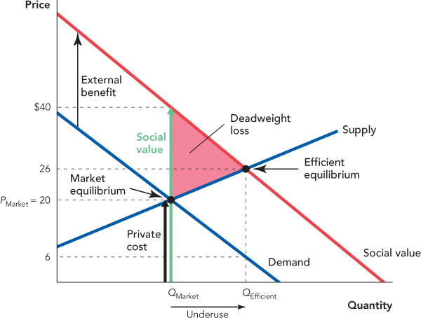
In Figure 10.3, for example, we show the demand and supply of vaccines. Demanders compare their private value of vaccines with their private costs and purchase QMarket units at the price PMarket. Vaccination, however, reduces the probability that a disease spreads so there are external benefits from vaccination. The social value curve counts all the benefits of vaccine use, the private value plus the external benefits, so the efficient quantity is found where the social value curve intersects the supply curve.
FIGURE 10.3

To see exactly why the market equilibrium is not efficient, consider in Figure 10.3 the private and social value of the QMarket unit of vaccination. This unit has a private cost of $20 (the black arrow labeled “Private cost”), but it has a social value of $40 (the green arrow labeled “Social value”). Thus, consuming more units would increase social surplus. Following this logic, you can see that increasing output increases social surplus so long as the social value of an additional flu shot exceeds the private cost, that is, so long as the social value curve is above the supply curve. Thus, to maximize social surplus, output should increase to QEfficient, the unit for which social value just equals the costs of production.
A final way of illustrating the underuse of vaccines is to notice that if people who got a flu shot did receive all the benefits of vaccination, then their demand curve would shift upward by $20 and would be the same as the social value curve. The market equilibrium would then be the same as the efficient equilibrium, that is, buyers would purchase QEfficient units. But for determining efficiency, who receives the benefits is irrelevant—benefits are benefits regardless of who receives them. Thus, QEfficient is the efficient quantity when vaccine users receive all of the benefits of vaccination and when they receive only some of the benefits—the only difference is that when other people receive some of the benefits, fewer people purchase flu shots, so QMarket < QEfficient.
CHECK YOURSELF
Question 10.1
 In our discussion of Pigouvian taxes, we assumed that the government set the correct tax to achieve the efficient equilibrium. What if government overshoots and adds a tax that is too high? Will the equilibrium quantity be higher or lower than the efficient equilibrium?
Question 10.2
 In our discussion of Pigouvian subsidies, we assumed that government set the correct subsidy amount to achieve the efficient equilibrium. What if the government undershoots and provides a subsidy that is too low? Will the equilibrium quantity be higher or lower than the efficient equilibrium?
The last way of thinking about the problem of external benefits also suggests one potential solution. If every time someone was vaccinated, they were given a subsidy of $20, the monetary equivalent of the external benefit, they would demand the amount QEfficient. Recall from Chapter 6 that we can analyze a subsidy by shifting up the demand curve by the amount of the subsidy. Thus, in Figure 10.3, notice that a subsidy set equal to the level of the external benefit would shift the demand curve up and increase the market quantity from QMarket to QEfficient. In other words, if set correctly, a subsidy will make the market equilibrium equal to the efficient equilibrium. In addition, unlike in Chapter 6 where we looked at subsidies on ordinary goods, a subsidy on a good with an external benefit will reduce deadweight loss, thereby increasing social surplus.
A Pigouvian subsidy is a subsidy on a good with external benefits.
A subsidy on a good with an external benefit is often called a Pigouvian subsidy, again after Pigou, who first discussed these issues. Another way of thinking about Pigouvian taxes and subsidies is to recall from Chapter 7 that market prices are signals. But when there are external costs or benefits, the market price sends the wrong signal. If there are external costs, the market price is too low, thus resulting in overconsumption. A Pigouvian tax increases the price so that the after-tax price sends the correct signal. Similarly, if there are external benefits, the market price is too high, thus resulting in underconsumption. A Pigouvian subsidy reduces the price so that the after-subsidy price sends the correct signal.
Let’s look in more detail at how to solve problems caused by external costs or benefits. We will discuss private solutions to problems created by externalities and three types of solutions involving government: taxes and subsidies (which we have mentioned already), command and control, and tradable permits.