10.3 Inference for Two Independent Proportions
 This page includes Statistical Videos
OBJECTIVES By the end of this section, I will be able to …
- Perform and interpret Z tests for p1−p2.
- Compute and interpret Z intervals for p1−p2.
- Use Z intervals for p1−p2 to perform two-tailed Z tests.
1 Independent Sample Z Tests for p1−p2
So far in this chapter, we have learned how to perform inference about population means. In this section, we learn how to perform hypothesis tests and construct confidence intervals about the difference between two population proportions. Recall that the sample proportion of success ˆp=x/n is the ratio of the number of successes x to the number of trials n in a binomial experiment.
In this section, we consider two independent samples, each of which yields a sample proportion: ˆp1=x1/n1 and ˆp2=x2/n2. For example, a recent survey found the sample proportion of males (sample 1) and females (sample 2) who agree that “technological changes will lead toward a future where people's lives are mostly better” to be
ˆp1=x1n1=335500=0.67
and
ˆp2=x2n2=255500=0.51
(See Example 15 for further details about these data.) Here, we are interested in performing inference for the difference in population proportions p1−p2, such as the difference in the proportions of all males and females who think technological change will lead to a better future. We use the difference in sample proportions ˆp1−ˆp2 as our point estimate of the difference in population proportions p1−p2, which is unknown. And just as in earlier sections where we investigated the sampling distribution of ˉx1−ˉx2 to perform inference on μ1−μ2, here we use the sampling distribution of ˆp1−ˆp2 to help us perform inference about p1−p2.
Developing Your Statistical Sense
Independent Samples Only
The inferential methods of this section are reserved for independent samples only. An example of a problem that would not use the methods of this section is the following: In the latest poll, suppose 45% of the respondents supported the Democratic candidate and 45% supported the Republican one. Because each respondent had to choose between the Democratic candidate and the Republican candidate, their respective poll numbers are not independent.
The distribution of all possible values of ˆp1−ˆp2 is called the sampling distribution of ˆp1−ˆp2, with mean p1−p2 and standard error
σˆp1−ˆp2=√p1(1−p1)n1+p2(1−p2)n2.
Let x1 and x2 denote the number of successes, and let n1−x1 and n2−x2 denote the number of failures in sample 1 and sample 2, respectively. The sampling distribution of ˆp1−ˆp2 is approximately normal when the number of successes and the number of failures in each sample are each at least 5, that is, when x1≥5, (n1−x1)≥5, x2≥5, and (n2−x2)≥5. Let q1=1−p1,q2=1−p2,ˆq1=1−ˆp1 and ˆq2=1−ˆp2.
Sampling Distribution of ˆp1−ˆp2
When two random samples are drawn independently from two populations, then the quantity
Z=(ˆp1−ˆp2)−(p1−p2)√p1q1n1+p2q2n2
has an approximately standard normal distribution when the following conditions are satisfied:
x1≥5,(n1−x1)≥5,x2≥5,(n2−x2)≥5
and where ˆp1 and n1 represent the sample proportion and sample size of the sample taken from population 1 with population proportion p1;ˆp2 and n2 represent the sample proportion and sample size of the sample taken from population 2 with population proportion p2; and q1=1−p1 and q2=1−p2.
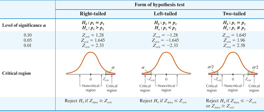
The three possible forms for the Z test for p1−p2 are as follows:
| H0 : p1=p2 | Ha:p1 > p2 | Right-tailed test |
| H0 : p1=p2 | Ha:p1 < p2 | Left-tailed test |
| H0 : p1=p2 | Ha:p1≠ p2 | Two-tailed test |
The null hypothesis asserts that H0 : p1=p2. We denote this common population proportion as p. The null hypothesis is assumed true, so the test statistic takes the following form:
Zdata=(ˆp1−ˆp2)−(p1−p2)√p1(1−p1)n1+p2(1−p2)n2=(ˆp1−ˆp2)−0√p1(1−p1)n1+p2(1−p2)n2=(ˆp1−ˆp2)√p(1−p)n1+p(1−p)n2=(ˆp1−ˆp2)√p(1−p)(1n1+1n2)
The common population proportion p is unknown, so we estimate it using the following pooled estimate of p:
ˆppooledx1+x2n1+n2
Note: As a check on your arithmetic, ˆppooled must also lie between ˆp1 and ˆp2.
Substituting this into the formula for the test statistic gives
Zdata=(ˆp1−ˆp2)√ˆppooled⋅(1−ˆppooled)(1n1+1n2)
Zdata measures the distance between the sample proportions. Extreme values of Zdata indicate evidence against the null hypothesis.
Hypothesis Test for the Difference in Two Population Proportions: Critical-Value Method
Suppose we have two independent random samples taken from two populations with population proportions p1 and p2, and the required conditions are met: x1≥5, (n1−x1)≥5, x2≥5, and (n2−x2) ≥ 5.
Step 1 State the hypotheses.
Use one of the forms from Table 12 (page 609). State the meaning of p1 and p2.
Step 2 Find Zcrit and state the rejection rule.
Use Table 12 on page 609.
Step 3 Calculate Zdata
Zdata=ˆp1−ˆp2√ˆppooled⋅(1−ˆppooled)(1n1+1n2)
where
ˆppooled=x1+x2n1+n2
Zdata follows an approximately standard normal distribution if the required conditions are satisfied.
Step 4 State the conclusion and the interpretation.
Compare Zdata with Zcrit.
|
EXAMPLE 15 Z test for p1−p2 using the critical-value method

In April 2014, the Pew Research Center published a report called U.S. Views of Technology and the Future,15 in which the results of a survey of Americans' views on the future of technology were examined. Among other questions, respondents were asked whether they agreed that “technological changes will lead toward a future where people's lives are mostly better.” The results are shown in Table 13. Assume the samples are independent.
| Males | Females | |
|---|---|---|
| Number agreeing | x1=335 | x2=255 |
| Sample size | n1=500 | n2=500 |
| Sample proportion | ˆp1=x1/n1=335/500=0.67 | ˆp2=x2/n2=255/500=0.51 |
| Population proportion | p1=? | p2=? |
- Find the point estimate of the difference in the population proportions of males and females, ˆp1−ˆp2.
- Compute the pooled estimate of the common proportion, ˆppooled.
- Calculate the value of the test statistic Zdata.
- Check whether the conditions for performing the Z test for p1−p2 are met.
- Test whether the population proportion of males who agree that technology will lead to a better future is greater than the population proportion of females who agree. Use the critical-value method at level of significance α=0.01.
Solution
- The point estimate is ˆp1−ˆp2=0.67−0.51=0.16
- ˆppooled=x1+x2n1+n2=335+255500+500=0.59
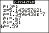 FIGURE 16 TI-83/84 results.
 - Zdata=ˆp1−ˆp2√ˆppooled⋅(1−ˆppooled)(1n1+1n2)=0.67−0.51√(0.59)(0.41)(1500+1500)≈5.1
- We check the conditions for performing the Z test for p1−p2. We have: x1=335≥5, x2=255≥5, n1−x1=500−335=165≥5, and n2−x2=500−255=245≥5. We may thus proceed with the hypothesis test.
- The Z test for p1≤p2 follows the steps below.
Step 1 State the hypotheses.
The key words “greater than,” together with the fact that sample 1 represents the males, indicate that we have a right-tailed test:
H0:p1=p2versusHa:p1>p2
where p1 and p2 represent the population proportion of males and females, respectively, who agree that technology will lead to a better future.
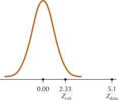 FIGURE 17 Zdata=5.1 is extreme, leading to rejection of H0.
Step 2 Find Zcrit and state the rejection rule.
For a right-tailed test with level of significance α=0.01, Table 12 gives us Zcrit=2.33 and our rejection rule: Reject H0 if Zdata≥2.33.
Step 3 Calculate Zdata.
From (c), we have Zdata≈5.1 (also see Figure 16).
Step 4 State the conclusion and the interpretation.
Zdata≈5.1≥2.33; therefore, reject H0 (see Figure 17). There is evidence at level of significance α=0.01 that the population proportion of males who agree that technology will lead to a better future is greater than the population proportion of females who agree.
NOW YOU CAN DO
Exercises 5–8.
We may also use the p-value method to perform the Z test for p1−p2.
Hypothesis Test for the Difference in Two Population Proportions: p-value Method
Suppose we have two independent random samples taken from two populations with population proportions p1 and p2, and the required conditions are met: x1≥5, (n1−x1) ≥ 5, x2≥5, and (n2−x2) ≥ 5.
- Step 1 State the hypotheses and the rejection rule.
Use one of the forms from Table 12. State the meaning of p1 and p2. The rejection rule is: Reject H0 if the p-value ≤α.
Step 2 calculate Zdata.
Zdata=ˆp1−ˆp2√ˆppooled⋅(1−ˆppooled)(1n1+1n2)
where ˆppooled=x1+x2n1+n2. If the required conditions are satisfied, Zdata follows an approximately standard normal distribution.
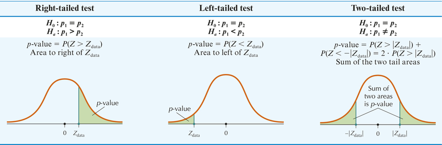
Step 3 Find the p-value.
Either use technology or calculate the p-value using one of the forms in Table 14.
Step 4 State the conclusion and the interpretation.
Compare the p-value with α.
|
EXAMPLE 16 Z test for p1−p2 using the p-value method

The General Social Survey tracks trends in American society through annual surveys. Married respondents were asked to characterize their feelings about being married. The results are shown here in a crosstabulation with gender. Test the hypothesis that the proportion of females who report being very happily married is smaller than the proportion of males who report being very happily married. Use the p-value method with level of significance α=0.05.
marriage
| Very happy | Pretty happy/ Not too happy |
Total | |
|---|---|---|---|
| Female | 257 | 166 | 423 |
| Male | 242 | 124 | 366 |
| Total | 499 | 290 | 789 |
Solution
From the crosstabulation, we assemble the statistics in Table 15 for the independent random samples of men and women.
| Sample size | Number very happy |
Sample proportion very happy | |
|---|---|---|---|
| Females (sample 1) | n1=423 | x1=257 | ˆp1=x1n1=257423≈0.6076 |
| Males (sample 2) | n2=366 | x2=242 | ˆp2=x2n2=257423≈0.6612 |
We first check whether the conditions for the Z test are valid: x1=257≥5, (n1−x1)=(423−257)=166≥5, x2=242≥5, and (n2−x2)=(366−242)=124≥5. We can therefore proceed.
Step 1 State the hypotheses and the rejection rule.
We are interested in whether the proportion of females who report being very happily married is smaller than that of males and because the females represent sample 1, the hypotheses are
H0:p1=p2Ha:p1<p2
Page 612where p1 and p2 represent the population proportions of all females and males, respectively, who report being very happily married. We will reject H0 if the p–value≤α=0.05.
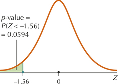 FIGURE 18 p-Value for left-tailed Z test.
Step 2 Find Zdata.
First, use the data from Table 15 to find the value of ˆppooled.
ˆppooled=x1+x2n1+n2=257+242423+366≈0.63245
Then
Zdata=(0.6076−0.6612)√0.63245⋅(1−0.63245)(1423+1366)≈−1.56
Step 3 Find the p-value.
Because it is a left-tailed test, the p-value is given by Table 14 as P(Z<Zdata)=P(Z<−1.56), as shown in Figure 18. This amounts to a Case 1 problem from Table 8 in Chapter 6 on page 357:
P(Z<−1.56)=0.0594
Step 4 State the conclusion and the interpretation.
The p-value=0.0594 is not less than or equal to α=0.05, so we do not reject H0. There is insufficient evidence that the proportion of females who report being very happily married is smaller than the proportion of males who do so.
Note: When the p-value is close to α, many data analysts prefer to simply assess the strength of evidence against the null hypothesis using criteria such as those given in Table 6 in Chapter 9 (page 514).
NOW YOU CAN DO
Exercises 9–12.
2 Independent Sample Z Interval for p1−p2
We have learned how to perform Z tests for p1−p2. Next, we learn how to use sample statistics to estimate p1−p2 using a confidence interval.
Confidence Interval for p1−p2
For two independent random samples taken from two populations with population proportions p1 and p2, a 100(1−α)% confidence interval for p1−p2 is given by
ˆp1−ˆp2±Zα/2√ˆp1⋅ˆq1n1+ˆp2⋅ˆq2n2
where ˆp1 and n1 represent the sample proportion and sample size of the sample taken from population 1 with population proportion p1; ˆp2 and n2 represent the sample proportion and sample size of the sample taken from population 2 with population proportion p2; ˆq1=1−ˆp1 and ˆq2=1−ˆp2, and the samples are drawn independently; and the following conditions are satisfied: x1≥5, (n1−x1)≥5, x2≥5, and (n2−x2)≥5.
Margin of Error E
The margin of error for a 100(1−α)% confidence interval for p1−p2 is given by
E=Zα/2⋅√ˆp1⋅ˆq1n1+ˆp2⋅ˆq2n2
EXAMPLE 17 Z confidence interval for p1−p2
Use the sample statistics from Example 15 to do the following:
- Calculate and interpret the margin of error E for confidence level 99%.
- Construct and interpret a 99% confidence interval for p1−p2.
Solution
The conditions for the confidence interval are the same as for the hypothesis test and were checked in Example 15.
ˆq1=1−ˆp1=1−0.67=0.33ˆq2=1−ˆp2=1−0.51=0.49.
From Table 1 in Chapter 8 on page 432, the Zα/2 value for a 99% confidence level is 2.576. Therefore, the margin of error is
E=Zα/2⋅√ˆp1⋅ˆq1n1+ˆp2⋅ˆq2n1=(2.576)√(0.67)(0.33)500+(0.51)(0.49)500≈0.079
The margin of error is 0.079, so we may estimate p1−p2 to within 0.079 with 99% confidence.
The point estimate is ˆp1−ˆp2=0.67−0.51=0.16. The 99% confidence interval is therefore
ˆp1−ˆp2±E=0.16±0.079=(0.081,0.239)
We are 99% confident that the difference in population proportions of males and females who agree that technology will lead to a better future lies between 0.081 and 0.239.
NOW YOU CAN DO
Exercises 13–18.
3 Use Z Confidence Intervals to Perform Z Tests for p1−p2
Given a 100(1−α)% Z confidence interval for p1−p2, we may perform two-tailed Z tests for various hypothesized values of p1−p2. If a proposed value lies outside the 100(1−α)% Z confidence interval for p1−p2, then the null hypothesis specifying this value would be rejected. Otherwise, do not reject the null hypothesis.
EXAMPLE 18 Using a Z interval for p1−p2 to perform Z tests about p1−p2
This example asks whether p1−p2 differs from (or is not equal to) a certain value, so we can use the Z confidence interval to test the hypotheses. Example 17 provided a 99% Z confidence interval for p1−p2, the difference in population proportions of males and females who agree that technology will lead to a better future, as (0.081, 0.239). Test, using level of significance α=0.01, whether the p1−p2 differs from these values: (a) 0.1, (b) 0.2, (c) 0.3.
Solution
H0:p1−p2=0.1 versus Ha:p1−p2≠0.1.
The hypothesized value 0.1 lies outside the interval (0.081, 0.239), so we reject H0.
H0:p1−p2=0.2 versus Ha:p1−p2≠0.2.
The hypothesized value 0.2 lies inside the interval, so we do not reject H0.
H0:p1−p2=0.3 versus Ha:p1−p2≠0.3.
The hypothesized value 0.3 lies outside the interval, so we reject H0.
NOW YOU CAN DO
Exercises 19–22.