14.6 Rank Correlation Test
OBJECTIVES By the end of this section, I will be able to …
- Perform the rank correlation test for paired data.
In Chapter 4, we learned how to calculate the correlation coefficient, which measures the strength of the linear association between two numerical variables. Here, in Section 14.6, we will learn how to calculate the rank correlation of two variables, which is the correlation of the variables based on ranks. We will also learn how to test whether the rank correlation between the variables is significant.
1 Rank Correlation Test
Similar to many nonparametric tests, the rank correlation test is a nonparametric hypothesis test that uses data that are ranked.
The rank correlation test (also called Spearman's rank correlation test) is based on the ranks of matched-pair data. This test may also be applied when the original data are ranks. In the rank correlation test we investigate whether two variables are related by analyzing the ranks of matched-pair data. The rank correlation test may also be used to detect a nonlinear relationship between two variables.
The hypotheses are
- H0:No rank correlation exists between the two variables.
- Hα:A rank correlation exists between the two variables.
The advantages to using the rank correlation test are that (a) it can be applied to ranked data, whereas linear correlation cannot, (b) it does not require normality, and (c) it can sometimes be used to uncover nonlinear relationships. A disadvantage of using the rank correlation test is that its efficiency rating is 0.91. That is, 100 data values are needed to achieve the same power that a linear correlation test achieves with only 91 data values, when the conditions for both tests are met.
To find the test statistic, we must calculate and square the paired differences of the ranks, a procedure shown in the next example.
EXAMPLE 19 Calculating the test statistic for the rank correlation test
femaleliteracy

The fertility rate is the mean number of children born to a typical woman in the country, and the female literacy rate is the percentage of women at least 15 years old who can read and write. The table contains the female literacy rate (in percent) and the fertility rate (in numbers of children) for a random sample of 10 countries.
| Country | Female literacy | Fertility |
|---|---|---|
| Afghanistan | 21 | 6.69 |
| India | 48 | 2.73 |
| Sudan | 51 | 4.7 2 |
| Saudi Arabia | 71 | 4.00 |
| South Africa | 86 | 2.20 |
| China | 87 | 1.73 |
| Israel | 94 | 2.41 |
| Italy | 98 | 1.28 |
| United States | 99 | 2.09 |
| Poland | 100 | 1.25 |
Calculate the test statistic for the rank correlation test, using the following steps:
- Rank the values of the first variable (female literacy) from lowest to highest.
- Rank the values of the second variable (fertility) from lowest to highest.
- For each subject (country), find the difference in ranks, d, and square the difference in ranks to get d2. Add up the d2-values to get ∑d2.
Complete the calculation of the test statistic rdata
rdata=1−6∑d2n(n2−1)
where n represents the sample size (number of matched pairs).
Solution
Table 15 contains the calculations needed to find rdata.
| Country | Female literacy |
Fertility | Literacy rank |
Fertility rank |
Difference d |
d2 |
|---|---|---|---|---|---|---|
| Afghanistan | 21 | 6.69 | 1 | 10 | −9 | 81 |
| India | 48 | 2.73 | 2 | 7 | −5 | 25 |
| Sudan | 51 | 4.72 | 3 | 9 | −6 | 36 |
| Saudi Arabia | 71 | 4.00 | 4 | 8 | −4 | 16 |
| South Africa | 86 | 2.20 | 5 | 5 | 0 | 0 |
| China | 87 | 1.73 | 6 | 3 | 3 | 9 |
| Israel | 94 | 2.41 | 7 | 6 | 1 | 1 |
| Italy | 98 | 1.28 | 8 | 2 | 6 | 36 |
| United States | 99 | 2.09 | 9 | 4 | 5 | 25 |
| Poland | 100 | 1.25 | 10 | 1 | 9 | 81 |
| Σd2=310 |
Because there are n=10 countries, the value of the test statistic is given by
rdata=1−6∑d2n(n2−1)=1−6(310)10(99)≈−0.8788
We now present the steps for performing the rank correlation test.
NOW YOU CAN DO
Exercises 9–12.
Rank Correlation Test
The sample paired data must be randomly selected. There is no requirement of normality.
- Step 1 State the hypotheses.
- H0:No rank correlation exists between the two variables.
- Hα:A rank correlation exists between the two variables.
- Step 2 Find the critical value and state the rejection rule.
- small-sample case (n≤30): Use Appendix Table K. Select the column with the appropriate level of significance α and the row with the appropriate sample size . The rejection rule for the rank correlation test is always to reject if or if .
- Large-sample case : A normal approximation is used. The critical value and the rejection rule are given in Table 16.
Table 14.76: Table 16 Critical values and rejection rule for the rank correlation test, large-sample caseLevel of significance α Critical value Rejection rule 0.10 Reject if 0.05 0.01 or if - Step 3 Find the value of the test statistic.
- Small-Sample Case : Use the following steps, preferably with a table similar to Table 15. If the original data already consist of ranks, then skip Steps a and b.
Rank the values of the first variable from lowest to highest.
Page 14-47- Rank the values of the second variable from lowest to highest.
- For each subject, find the difference in ranks, , and square the difference in ranks to get . Add up the -values to get .
Complete the calculation of the test statistic:
where represents the sample size (number of matched pairs).
- Large-sample case : Use Steps a–d from the small-sample case. However, we are using a normal approximation, so the test statistic is called .
- Small-Sample Case : Use the following steps, preferably with a table similar to Table 15. If the original data already consist of ranks, then skip Steps a and b.
Step 4 state the conclusion and the interpretation.
Compare the test statistic with the critical value, using the rejection rule.
EXAMPLE 20 Performing the rank correlation test
Use the data in Example 19 to test whether a rank correlation exists between female literacy and fertility. Use level of significance .
Solution
The data come from a random sample, so we may proceed with the hypothesis test.
- Step 1 State the hypotheses.
- Step 2 Find the critical value and state the rejection rule. There are countries in the data set in Table 15, so we apply the small-sample case (). Use Appendix Table K. We select the column with level of significance and the row with . Our critical value is (see Figure 22). We will reject , if or if .
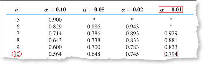 FIGURE 22 Finding the critical value for the rank correlation test.
 - Step 3 Find the value of the test statistic . In Example 19, we found .
- Step 4 State the conclusion and the interpretation. Because , our conclusion is to reject . There is evidence for a rank correlation between female literacy and fertility. Because is negative, the association between female literacy and fertility is a negative relationship. That is, as female literacy increases, fertility tends to decrease, and vice versa.
NOW YOU CAN DO
Exercises 13–20.
EXAMPLE 21 Rank correlation test: Large-sample case
Expand the previous example from countries to a random sample of countries, and conduct the same hypothesis test, using the same level of significance . Assume that the 37 countries yield a test statistic of .
Solution
The expanded data set comes from a random sample, so we proceed with the hypothesis test.
- Step 1 State the hypotheses.
Step 2 Find the critical value and state the rejection rule. There are now countries, so we apply the large-sample case . With level of significance , we find our critical value from Table 16:
We will reject if or if .
- Step 3 Find the value of the test statistic . We use the instructions provided in the Step-by-Step Technology Guide at the end of this section. Figure 23 shows the Minitab results, with denoted as “.” Although Minitab thus identifies the statistic as the linear correlation coefficient for numerical data that we learned in Chapter 4, this statistic is nevertheless equal to the rank correlation coefficient, because it is based on ranks.
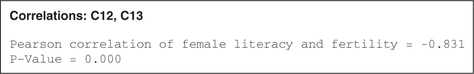 FIGURE 23 Minitab results.
 - Step 4 State the conclusion and the interpretation. Because , we reject , just as we did for the small-sample case. There is evidence for a rank correlation between female literacy and fertility.
EXAMPLE 22 Using rank correlation to detect a nonlinear pattern
scrabble
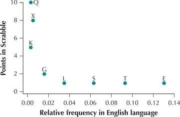
In the Chapter 13 Case Study, “How Fair Is the Scoring in Scrabble?” we noted from a scatterplot of Scrabble point values versus English-language letter frequencies that the relationship between the variables was not linear. Thus, we could not use a linear regression analysis. However, we can use rank correlation to test whether the two variables are associated, because linearity is not a condition for applying the rank correlation test.
For the following random sample of letters, use the rank correlation test to investigate whether an association exists between English-language frequencies and Scrabble point values. Use level of significance . Note from Figure 24 that the relationship between the variables is certainly nonlinear.
| Letter | Frequency | Scrabble points |
|---|---|---|
| Q | 0.003 | 10 |
| L | 0.035 | 1 |
| G | 0.016 | 2 |
| E | 0.130 | 1 |
| X | 0.005 | 8 |
| T | 0.093 | 1 |
| S | 0.063 | 1 |
| K | 0.003 | 5 |
Solution
The data come from a random sample, so we may proceed with the hypothesis test.
- Step 1 State the hypotheses.
- Step 2 Find the critical value and state the rejection rule. There are letters in the random sample, so we apply the small-sample case . Using Appendix Table K, we select the column with level of significance and the row with . Our critical value is . We will reject if or if .
- Step 3 Find the value of the test statistic. See Table 17.Table 14.78: Table 17 Table of calculations to find
Letter Frequency Scrabble
pointsFrequency
rankScrabble
rankDifference Q 0.003 10 1.5 8 −6.5 42.25 L 0.035 1 5 2.5 2.5 6.25 G 0.016 2 4 5 −1 1 E 0.130 1 8 2.5 5.5 30.25 X 0.005 8 3 7 −4 16 T 0.093 1 7 2.5 4.5 20.25 S 0.063 1 6 2.5 3.5 12.25 K 0.003 5 1.5 6 −4.5 20.25 There are letters in the sample, so the value of the test statistic is given by
- Step 4 State the conclusion and the interpretation. Because , we reject . There is evidence for a rank correlation between the frequency of letters in the English language and the number of points each letter is worth in the game of Scrabble. Because is negative, the relationship is also negative. That is, high point values are associated with low frequency in English, and vice versa.
 Does a rank correlation exist between the 2007 and 2014 vehicle Gas Mileages?
We return to the random sample of 14 vehicle gas mileages (shown below in Table 18) for the Chapter 14 Case Study. Recall that we are dealing with matched-pair data, comparing the miles per gallon (mpg) for the same vehicles from two different years. In Section 14.2, we tested whether the median gas mileage increased. However, the data take the form of matched pairs, so we can also investigate whether an association exists between the 2007 and 2014 vehicle gas mileages using the rank correlation test. Test whether a rank correlation exists between the 2007 mpg and the 2014 mpg, using level of significance .
| Make | Model | Combined mpg for 2007 |
Combined mpg for 2014 |
2000 mpg rank |
2007 mpg rank |
Difference
|
|
|---|---|---|---|---|---|---|---|
| Chevrolet | Tahoe | 17 | 17 | 4.5 | 3 | 1.5 | 2.25 |
| Chevrolet | Suburban | 17 | 17 | 4.5 | 3 | 1.5 | 2.25 |
| Dodge | Caravan | 21 | 20 | 8.5 | 8 | 0.5 | 0.25 |
| Ford | Explorer | 17 | 19 | 4.5 | 6.5 | −2 | 4 |
| Ford | F150 Pickup | 16 | 18 | 1 | 5 | −4 | 16 |
| Ford | Mustang | 17 | 19 | 4.5 | 6.5 | −2 | 4 |
| Ford | Ta u r u s | 23 | 21 | 10 | 9 | 1 | 1 |
| GMC | Savana Cargo | 17 | 16 | 4.5 | 1 | 3.5 | 12.25 |
| GMC | Yukon X L | 17 | 17 | 4.5 | 3 | 1.5 | 2.25 |
| Subaru | Forester | 25 | 27 | 12 | 12 | 0 | 0 |
| Subaru | Impreza | 25 | 27 | 12 | 12 | 0 | 0 |
| Subaru | Legacy | 25 | 27 | 12 | 12 | 0 | 0 |
| Toyota | Corolla | 36 | 35 | 14 | 14 | 0 | 0 |
| Toyota | Ta com a | 21 | 23 | 8.5 | 10 | −1. 5 | 2.25 |
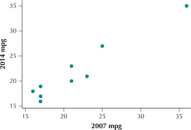
What Result Might We Expect?
Consider Figure 25, which shows a scatterplot of the 2014 mpg versus the 2007 vehicle mpg. There appears to be a rather strong positive relationship between the two variables, and thus a strong correlation. We would therefore expect to reject the null hypothesis that there is no rank correlation.
Solution
The data come from a random sample of matched pairs, so we may proceed with the hypothesis test.
- Step 1 State the hypotheses.
- Step 2 Find the critical value and state the rejection rule. There are vehicles in the data set, so we apply the small-sample case . In Appendix Table K we select the column with level of significance and the row with . Our critical value is . We will reject if or if .
Step 3 Find the value of the test statistic . We use Table 18 to find We have
Then, because there are vehicles, the value of the test statistic is given by
- Step 4 State the conclusion and the interpretation. Because , we reject . Evidence exists for a rank correlation between the 2007 vehicle mpg and the 2014 vehicle mpg. Because is positive, the association between 2007 and 2014 vehicle mpg is a positive relationship. In other words, vehicles that had low gas mileage in 2007 tended to have low gas mileage in 2014, while the vehicles that had high gas mileage in 2007 tended to have high gas mileage in 2014.