14.7 Runs Test for Randomness
OBJECTIVES By the end of this section, I will be able to …
- Perform the runs test for randomness.
Recall from Chapter 13 that one of the assumptions for the linear regression model was that the values of the response variable y were independent. We checked this assumption using a scatterplot of the residuals against the fitted values; if systematic curvature was present, then the assumption was violated. Here, in Section 14.7, we learn a hypothesis test for checking this assumption, called the runs test for randomness.
1 Runs Test for Randomness
In contrast to the other sections in this chapter, in this section we look upon our data set as a sequence. The first observation is considered to occur before the second, which is before the third, and so on. That is, a sequence is an ordered data set.
 Note that we are considering the data set to be a sequence (time-ordered) only for the application of the runs test for randomness. We are not suggesting that the data set itself is necessarily time-ordered.
The runs test for randomness helps us determine whether the data in the sequence are random or whether there is a pattern in the sequence. The runs test applies to data that have two possible outcomes (such as female or male) or data that can be reexpressed as one of two outcomes (such as correct or incorrect answers on a multiple-choice quiz). The runs test works by counting the number of runs in the data set.
A sequence is an ordered data set. A run is a sequence of observations sharing the same value (of two possible values), preceded or followed by data having the other possible value or by no data at all. The runs test for randomness tests whether the data in a sequence are random or whether there is a pattern in the sequence.
For example, suppose that we are noting the gender (F = female, M = male) of the first 16 students to enter your statistics classroom today as they walk in the door. Here are two possible sequences:
| Sequence 1: | F | F | F | F | F | F | F | F | M | M | M | M | M | M | M | M |
| Sequence 2: | F | M | F | M | F | M | F | M | F | M | F | M | F | M | F | M |
In the first sequence, there is a run of eight females, followed by a run of eight males. The eight females form a run because they represent a sequence of observations sharing the same value: F. Similarly, the eight males form a run. In Sequence 2, we note that the genders are alternating. The first data value F is followed immediately by an observation with a different value: M. Thus, the first data value itself forms a run. Similarly, each of the remaining observations forms a run of length 1.
The following notation is used in conducting a runs test for randomness:
- n1=the number of observations having the first distinct outcome
- n2=the number of observations having the second distinct outcome
- n=the total number of observations in the data set, n=n1+n2
- G=the number of runs in the sequence
EXAMPLE 23 Notation used for the runs test for randomness
The following sequence represents the genders of 20 students in a statistics class recorded as they enter the classroom:
| F | F | M | M | M | F | F | F | M | F | F | F | M | M | F | F | M | F | F | M |
Calculate the values of n1, n2, n, and G.
Solution
There are n1=12 females and n2=8 males, so that n=n1+n2=12+8=20. There are G=10 runs.
NOW YOU CAN DO
Exercises 5–8.
If the number of runs is too low or too high, this is evidence that a pattern exists in the data set. If the number of runs is neither too high nor too low, this is evidence that no time-ordered pattern exists in the data set, which may then be considered random. Thus, the runs test for randomness tests whether the number of runs is either too high or too low. There are large- and small-sample cases for the test statistic and the critical values for the runs test for randomness, as shown in the following steps.
Runs Test for Randomness
Two conditions are necessary for the runs test: (a) the data are ordered, and (b) each data value represents one of two distinct outcomes (such as female or male).
- Step 1 State the hypotheses.
- H0:The sequence of data is random.
- Hα:The sequence of data is not random.
- Step 2 Find the critical values, and state the rejection rule.
Small-Sample Case (n1≤20, n2≤20, and level of significance α=0.05): Use Appendix Table L. Note that the table is applicable only for level of significance α=0.05. Find the row with the appropriate value of n1 and the column with the appropriate value of n2. The two values at the intersection of this row and column represent the lower critical value Gcrit, lower and the upper critical value Gcrit, upper. The rejection rule is to reject H0 if Gdata≤Gcrit, lower or if Gdata≤Gcrit, upper.
Page 14-57- Large-Sample Case (n1>20 or n2>20): A normal approximation is used. See Table 19.Table 14.96: Table 19 Critical values and rejection rule for the runs test, large-sample case
Level of
significance αCritical value Zcrit Rejection rule 0.10 1.645 Reject H0 if 0.05 1.96 Zdata≤−Zcrit 0.01 2.58 or if Zdata≥Zcrit
Step 3 Find the value of the test statistic.
- Small-Sample Case (n1≤20 and n2≤20): The test statistic Gdata is simply the number of runs, G:
Gdata=G
- Large-Sample Case (n1>20 or n2>20): First find the number of runs G. Then calculate the following quantities:
μG=2n1n2n1+n2+1σG=√(2n1n2)(2n1n2−n1−n2)(n1+n2)2(n1+n2−1)
Finally, the test statistic is Zdata:
Zdata=G−μGσG
- Small-Sample Case (n1≤20 and n2≤20): The test statistic Gdata is simply the number of runs, G:
Step 4 State the conclusion and the interpretation.
Compare the test statistic with the critical value, using the rejection rule.
EXAMPLE 24 Conducting the runs test for randomness
Test whether the sequence from Example 23 is random by conducting the runs test for randomness, using level of significance α=0.05.
Solution
We know that the data are time-ordered, and that each data value represents one of two distinct outcomes. We may thus proceed with the hypothesis test.
- Step 1 State the hypotheses.
- H0:The sequence of data is random.
- Hα:The sequence of data is not random.
Step 2 Find the critical values, and state the rejection rule. We have n1=12 females and n2=8 males, so the small-sample case applies (n1≤20 and n2≤20). In Appendix Table L we find the row with n1=12 and the column with n2=8, giving us the critical values Gcrit, lower=6 and Gcrit, upper=16 (see Figure 26). We will reject H0 if Gdata≤6 or if Gdata≥16.
Page 14-58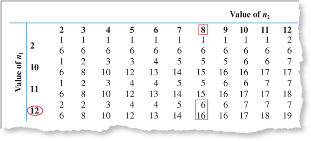 FIGURE 26 Finding the critical values for the runs test for randomness.
- Step 3 Find the value of the test statistic. We have the small-sample case, so the test statistic Gdata is simply the number of runs, G:
Gdata=G=10
- Step 4 State the conclusion and the interpretation. Because Gdata=10 is not ≤6 and is not ≥16, we do not reject H0. There is insufficient evidence that the sequence is not random.
NOW YOU CAN DO
Exercises 9–20.
The runs test may also be used for numerical data, as long as the numerical data are classified into two categories, as shown in the following example.
EXAMPLE 25 Runs test for randomness of numerical data classified into categories
The weather station at the University of Missouri at Columbia publishes daily information on the amount of rain that falls at Sanborn Field at the university. The following 62 observations represent the daily rainfall information for the months of July and August 2008. For example, on July 1 the weather station reported 0.00 inch of rain, and on July 2 the weather station reported 0.37 inch of rain. We categorize each day's rainfall as follows: N = no rain falling, and R = some rain falling. Test whether the sequence is random by conducting the runs test for randomness, using level of significance α=0.10.
| N | R | R | N | N | N | N | R | R | N | N | R | N | N | N | N | N | N | N | N | N | R | N | R | R | N | R | R | N | R | R |
| N | N | N | N | N | N | N | N | N | N | N | R | N | R | N | N | N | N | N | R | R | R | N | N | N | N | N | R | N | N | N |
Solution
The data are ordered, because they are arranged from July 1 to August 31, 2008. Also, each data value represents one of two distinct outcomes: some rain or no rain. We may thus proceed with the hypothesis test.
Step 1 State the hypotheses.
- H0:The sequence of data is random.
- Hα:The sequence of data is not random.
Page 14-59- Step 2 Find the critical values, and state the rejection rule. We have n1=18 rainy days and n2=44 days with no rain. Because n2>20, the large-sample case applies. From Table 19, the critical value is 1.645, and we will reject H0 if Zdata≤−1.645 or if Zdata≥1.645.
Step 3 Find the value of the test statistic. We have n=n1+n2=18+44=62, and there are G=23 runs. Then
μG=2n1n2n1+n2+1=2(18)(44)18+44+1≈26.5484σG=√(2n1n2)(2n1n2−n1−n2)(n1+n2)2(n1+n2−1)=√[2(18)(44)][(18)(44)−18−44](18+44)2(18+44−1)≈3.2065
Finally, the test statistic is
Zdata=23−26.54843.2065≈−1.1066
- Step 4 State the conclusion and the interpretation. Because –1.1066 is not less than –1.645 and is not more than 1.645, we do not reject H0. There is insufficient evidence that the sequence is not random.
The runs test for randomness may also be used to test the independence assumption for linear regression data, as shown in the following example. The important thing to remember is that the runs test should be applied to the residuals, which are ordered by the size of the fits (ˆy).
EXAMPLE 26 Using the runs test for linear regression
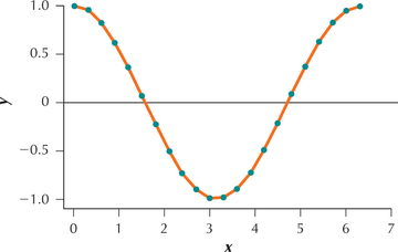
Consider the following ordered bivariate data set and the accompanying scatterplot (Figure 27). We are interested in performing linear regression of the y variable on the x variable. Make a scatterplot of the residuals (y-ˆy) versus the fts (ˆy). Classify the residuals as being either positive (P) or negative (N). Then evaluate the independence assumption for the linear regression model by performing the runs test for randomness on the residuals, ordered by the fits.
| x | y | x | y |
|---|---|---|---|
| 0.0 | 1.00000 | 3.3 | −0.98748 |
| 0.3 | 0.95534 | 3.6 | −0.89676 |
| 0.6 | 0.82534 | 3.9 | −0.72593 |
| 0.9 | 0.62161 | 4.2 | −0.49026 |
| 1.2 | 0.36236 | 4.5 | −0.21080 |
| 1.5 | 0.07074 | 4.8 | 0.08750 |
| 1.8 | −0.22720 | 5.1 | 0.37798 |
| 2.1 | −0.50485 | 5.4 | 0.63469 |
| 2.4 | −0.73739 | 5.7 | 0.83471 |
| 2.7 | −0.90407 | 6.0 | 0.96 017 |
| 3.0 | −0.98999 | 6.3 | 0.99986 |
Solution
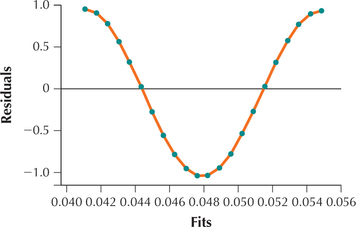
The scatterplot of the residuals versus the fts is shown in Figure 28.
What Results Might We Expect?
When applied to linear regression analysis, the runs test for randomness tests whether a pattern exists in the residuals. Do you observe a pattern in the scatterplot of the residuals (Figure 28)? If so, then what might we expect our conclusion to be for the runs test? Yes, there appears to be a descending and then ascending pattern in the data (In fact, can you discern the exact relationship between x and y?), and thus we expect to reject the null hypothesis that the data are random
By examining Figure 28, we can classify the residuals from left to right as positive or negative, giving us:
| P | P | P | P | P | P | N | N | N | N | N | N | N | N | N | N | P | P | P | P | P | P |
The residuals are ordered by the size of the fts, and we have classified each residual into one of two distinct outcomes. Thus, we may proceed with the hypothesis test.
- Step 1 State the hypotheses.
- H0:The sequence of residuals is random.
- Hα:The sequence of residuals is not random.
- Step 2 Find the critical values, and state the rejection rule. We have n1=12 positives and n2=10 negatives, so the small-sample case applies (n1≤20 and n2≤20). From Appendix Table L we find our critical values Gcrit, lower=7 and Gcrit, upper=17. We will reject H0 if Gdata≤7 or if Gdata≥17.
- Step 3 Find the value of the test statistic. We have the small-sample case, so the test statistic Gdata is simply the number of runs, G:
Gdata=G=3
- Step 4 State the conclusion and the interpretation. Because G=3 is less than 7, we reject H0. Evidence exists that the sequence of residuals is not random. The residuals are nonrandom, so the independence assumption for the linear regression model is violated, and we should not proceed with a linear regression analysis.
By the way, have you guessed the equation of the pattern shown in Figures 27 and 28? The relationship between x and y is y=cos(x).