3.1 Measures of Center
 This page includes Statistical Videos
OBJECTIVES By the end of this section, I will be able to …
- Calculate the mean for a given data set.
- Find the median, and describe why the median is sometimes preferable to the mean.
- Find the mode of a data set.
- Describe how skewness and symmetry affect these measures of center.
Do you like to make money? Then you might want to stay in school and finish your Bachelor's degree. The Pew Research Center reports that the median annual earnings among young people ages 25-32 with a Bachelor's degree was $45,500, compared with $30,000 for those who did not finish their college degree (Source: Pew Research Center: The Rising Cost of Not Going to College1). The $45,500 is a sample median, which was calculated from the sample taken by the researchers. As such, it summarizes the earnings of over 1000 different young people from all over the country. In Chapter 3, we learn how to do this: to summarize an entire dataset with just a few numbers. In Section 3.1, we will learn about three numerical measures that tell us where the center of the data lies: the mean, the median, and the mode.
1 The Mean
The most well-known and widely used measure of center is the mean. In everyday usage, the word average is often used to denote the mean.
The mean is often called the arithmetic mean.
To find the mean of the values in a data set, simply add up all the numbers and divide by how many numbers you have.
EXAMPLE 1 Calculating the population mean
The Web site CNET.com provides reviews and prices for gadgets and electronics, including cell phones. In Table 1, you will find all eight of the cell phones in CNET's “Editors' Picks” for June 27, 2014. Recall from Chapter 1 that a population is the collection of all elements of interest in a particular study. Thus, the data in Table 1 represents a population. Find the mean price of all the cell phones.
| Samsung Galaxy S5 Standard | $200 |
| Samsung Galaxy S5 Active | $200 |
| Sony Xperia Z2 | $600 |
| Nokia Lumia Icon | $200 |
| LG G3 | $800 |
| Apple iPhone 5s | $250 |
| HTC One M8 | $200 |
| Samsung Galaxy Note 3 | $300 |
Solution
To find the mean, we add up the prices of all eight cell phones and divide by the number of phones:
Mean Cell Phone price=200+200+600+200+800+250+200+3008=$343.75
The population mean price for all eight cell phones is $343.75.
NOW YOU CAN DO
Exercises 13–18.
YOUR TURN#1
Table 2 contains the number of tropical storms reported by the National Oceanic and Atmospheric Administration for 2006-2013. All years in this period are represented, so this can be considered a population. Find the population mean number of tropical storms.
| Year | 2006 | 2007 | 2008 | 2009 | 2010 | 2011 | 2012 | 2013 |
|---|---|---|---|---|---|---|---|---|
| Tropical storms | 10 | 15 | 16 | 9 | 19 | 19 | 19 | 14 |
(The solution is shown in Appendix A.)
Before we proceed, we need to learn some notation.
Notation
Statisticians like to use specialized notation. It is worth learning because it saves a lot of writing, and certain concepts can best be understood by using this special notation.
- The population size, the number of observations in your population, is always denoted as N. We have a population with eight observations in Example 1, so N=8.
- The sample size, which refers to how many observations you have in your sample data set, is always denoted as n.
- The shorthand notation for “the sum of all the data” is ∑x, where x refers to the data, and ∑ (capital sigma), which is the Greek letter for “S,” stands for “Summation.” Note in Example 1 that we added up the prices of all the cell phones. This summing is denoted as ∑x.
- The population mean is denoted as μ (pronounced “mew”), which is the Greek letter for m. As we saw in Example 1, to calculate the population mean, we add up all the data and divide by the population size, . Thus, the formula for the population mean is:
For Example 1, we therefore have:
- The sample mean is denoted as (pronounced “x-bar”). You should try to commit this to long-term memory because may be the most important symbol used in this book and will return again and again in nearly every chapter. The sample mean is calculated just like the population mean, except that we divide by the sample size instead of the population size . Thus, the formula for the sample mean is:
EXAMPLE 2 Calculating the sample mean
Suppose the cell phones in Table 3 represent a random sample of size four from the population in Table 1. Calculate the sample mean price of this sample of cell phones.
| Samsung Galaxy S5 Active | $200 |
| Sony Xperia Z2 | $600 |
| Apple iPhone 5s | $250 |
| Samsung Galaxy Note 3 | $300 |
Solution
The sample mean price of this sample of four cell phones is calculated like this:
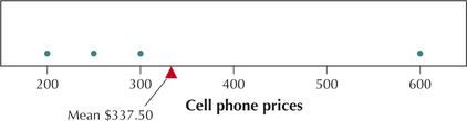
The sample mean cell phone price for this particular sample is $337.50. Of course, a different sample would have yielded a different value for .
NOW YOU CAN DO
Exercises 19–24.
YOUR TURN#2
Suppose we took a sample of size three instead and obtained the same sample as in Table 3, except that the Sony Xperia Z2 was not included.
- Would you expect that the sample mean price would be higher or lower than $337.50? Explain.
- Calculate the sample mean price for the sample of three cell phones. Was your intuition in (a) confirmed?
(The solutions are shown in Appendix A.)
What Does This Number Mean?
The Mean as the Balance Point of the Data
Let's explore our sample cell phone price data a bit further. Consider the dotplot of the cell phone prices in Figure 1. To find out where the mean price lies on this number line, imagine that the dots are little blocks on a ruler or a seesaw and that you must decide where to place the support (like the triangle in Figure 1) so that the ruler balances perfectly. The place where the data set balances perfectly is the location of the mean. Placing the fulcrum too far to the right or left would create an imbalance. This data set balances precisely at the sample mean,
Developing Your Statistical Sense
Checking Your Results Against Experience and Common Sense
When you have found the balance point, you have found the mean. When you calculate the mean, or have a computer or calculator do it for you, don't just accept whatever value pops out. Make sure the result makes sense. Because the mean always indicates the place where the data values are in balance, the mean is often near the center of the data. If the value you have calculated lies nowhere near the center of the data, then you may want to check your calculations.
For example, suppose we were finding the mean of the cell phone data, and we accidentally entered 6000 instead of 600 for the price of the Sony Xperia Z2. Then, our value for the mean resulting from this incorrect calculation would be
The mean price cannot equal $1687.50 because all the values in the data set are less than $1687.50. The mean can never be larger or smaller than all the values in the data set.
Don't automatically accept the result you get from a computer or calculator. Remember GIGO: Garbage In Garbage Out. If you enter the wrong data, the calculator or computer will not bail you out. Human error is one reason for the explosion of faulty statistical analyses in the newspapers and on the Internet. Now more than ever, data analysts must use good judgment. When you calculate a mean, always have an idea of what you expect the sample mean to be, that is, at least a ballpark figure.
For calculating the mean, we will adopt the convention of rounding our final calculation, if necessary, to one more decimal place than that in the original data.
The Mean Is Sensitive to Extreme Values
One drawback of using the mean to measure the center of the data is that the mean is sensitive to the presence of extreme values in the data set. We illustrate this phenomenon with the following example.
EXAMPLE 3 Sensitivity of the mean to extreme values
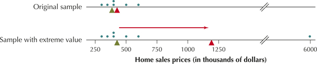
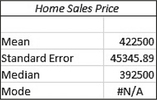
Table 4 contains a sample of six home sales prices for Broward County, Florida, for June 27, 2014. We want to get an idea of the typical home sales price in Broward County.
- Find the mean sales price of the homes in Table 4.
- Suppose we add a seventh home in Hillsborough Beach, selling for $6 million. Calculate the mean sales price of all seven homes. Comment on how the extreme value affected the mean sales price.
homesales
| Location | Price |
|---|---|
| Pembroke Pines | $300,000 |
| Weston | $350,000 |
| Hallandale | $360,000 |
| Miramar | $425,000 |
| Davie | $500,000 |
| Fort Lauderdale | $600,000 |
Solution
The mean sales price of the homes in Table 4 is:
- Now, suppose that we append a seventh home to our sample: a home in Hillsborough Beach listed for $6 million, which is much more expensive than any of the other homes in the sample. Recalculating the mean, we get
Note that the mean sales price nearly tripled from $422,500 to $1,220,000 when we added this extreme value. Also, this new mean is much higher than every price in the original sample. Thus, it is highly unlikely that this new mean of about $1.2 million is representative of the typical sales price of homes in Broward County. This example shows how the mean is sensitive to the presence of extreme values. For situations like this, we prefer a measure of center that is not so sensitive to extreme values. Fortunately, the median is just such a measure.
NOW YOU CAN DO
Exercises 25–30.
2 The Median
Recall that the median strip on a highway is the slice of land in the middle of the two lanes of the highway. In statistics, the median of a data set is the middle data value when the data are put into ascending order. There are two cases, depending on whether the sample size is odd or even.
The Median
The median of a data set is the middle data value when the data are put into ascending order. Half of the data values lie below the median, and half lie above.
- If the sample size is odd, then the median is the middle value and lies at the position when the data are put in ascending order.
- If the sample size is even, then the med values that the median is the mean of the two middle data values that lie on either side of the position.

The case when the sample size is even is clear if you hold up four fingers on one hand. Notice that there is no unique finger in the middle. No middle value exists when the sample size is even, so we take the two data values in the middle and split the difference.
The Median Is Not Sensitive to Extreme Values
Unlike the mean, the median is not sensitive to extreme values. If the expensive home is included in the sample, the median price should not change much, even though, as we saw in Example 3, the mean sales price nearly tripled. Let's look at an example of how this would occur.
EXAMPLE 4 Median is not sensitive to extreme values
Show that the median is not sensitive to extreme values by doing the following:
- Find the median sales price of the homes in Table 4.
- Add the seventh home in Hillsborough Beach, selling for $6 million. Calculate the median sales price of all seven homes.
Because the median is not sensitive to extreme values, we say that it is a robust, or resistant, measure of center. The mean is neither robust nor resistant.
Solution
- Fortunately, the data are already presented in ascending order in the table. Because is even, the median is the mean of the two data values that lie on either side of the position. That is, the median is the mean of the 3rd and 4th data values, $360,000 and $425,000. Splitting the difference between these two, we get
We note that, in Table 4, there are exactly as many homes with prices lower than $392,500 as homes with prices higher than $392,500.
- Now, what happens to the median when we add in the $6 million home from Hillsborough Beach? Because is odd, the median is the unique observation, given by the home in Miramar for $425,000. The extreme value increased the median only from $392,500 to $425,000. In Example 3, we showed that the value of the mean price nearly tripled when the expensive home was added. Thus, the median home sales price is a better measure of center because it more accurately reflects the typical sales prices of homes in Broward County.
NOW YOU CAN DO
Exercises 31–36.
![]() The Mean and Median applet allows you to insert your own data values and see how changes in these values affect both the mean and the median.
The Mean and Median applet allows you to insert your own data values and see how changes in these values affect both the mean and the median.
EXAMPLE 5 Using technology to find the mean and median
 Note that the formula gives the position, not the value, of the median. For example, the median home sales price for Table 4 is not
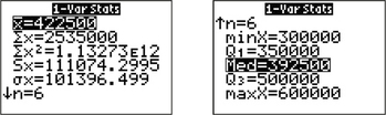
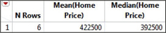
Find the mean and median of the home sales prices in Table 4, using (a) the TI-83/84, (b) Excel, (c) Minitab, and (d) JMP.
Solution
Using the instructions in the Step-by-Step Technology Guide on page 117, we get the following output:
- The first TI-83/84 screen shows and . The second screen shows the median, .
- The mean and median are shown in the Excel output.
 Page 114
 - The mean and median are shown in the Minitab output.

- The mean and median are shown in the JMP output.
3 The Mode
Sometimes the mode does not indicate the center of a data set. For example, suppose we have the following set of biology lab scores: 60, 80, 100, 100. The mode is 100, but it is not near the center of the data.
A third measure of center is called the mode. French speakers will recognize that the term mode in French refers to fashion. The popularity of clothing, cosmetics, music, and even basketball shoes often depends on just which style is in fashion. In a data set, the value that is most “in fashion” is the value that occurs the most.
The mode of a data set is the data value that occurs with the greatest frequency.
EXAMPLE 6 Finding the mean, median, and mode: Music videos
The Web site MTV.com contains music videos for many performers. Table 5 provides the number of music videos available for download for four performers, as of May 21, 2012. Find the (a) mean, (b) median, and (c) mode number of music videos.
| Performer | Music Videos |
|---|---|
| Michael Jackson | 31 |
| Taylor Swift | 26 |
| Usher | 26 |
| Katy Perry | 15 |
Solution
- The sample mean number of music videos is
The mean number of music videos is 24.5.
- Because is even, the median is the mean of the two middle data values:
- The mode is the data value that occurs with the greatest frequency. Two performers have 26 music videos: Taylor Swift and Usher. No other data value occurs more than once. Therefore, the mode is 26 music videos, as shown in Figure 3.
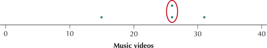 FIGURE 3 Dotplot of music videos, showing 26 as the mode.
NOW YOU CAN DO
Exercises 37–40.
YOUR TURN#3
Take a sample from Table 2 that consists of the number of tropical storms from the even-numbered years. Find the mean, median, and mode number of tropical storms.
(The solutions are shown in Appendix A.)
One of the strengths of the mode is that it can also be used with categorical, or qualitative, data. Suppose you asked your friends to name their favorite flower. Six of them answered “rose,” three answered “lily,” and one answered “daffodil.” Note that these data are categorical, not numerical. The most frequently occurring flower is “rose”; therefore, the rose represents the mode of the variable favorite flower. Unfortunately, we cannot use arithmetic with categorical variables, and thus the mean or median for this variable cannot be found.
It may happen that no value occurs more than once, in which case we say there is no mode. On the other hand, more than one data value could occur with the greatest frequency, in which case we would say there is more than one mode. Data sets with one mode are unimodal; data sets with more than one mode are multimodal.
 What If Scenario
Consider Example 6 once again. Now imagine: what if there was an incorrect data entry, such as a typo, and the number of Michael Jackson's videos was greater than 31 by some unspecified amount?
Describe how and why this change would have affected the following, if at all:
- The mean number of music videos
- The median number of music videos
- The mode number of music videos
Solution
- Consider Figure 4, a dotplot of the number of music videos, with the triangle indicating the mean, or balance point, at 24.5. Recall that this represents the balance point of the data. As the number of Michael Jackson's videos increases (arrow), the point at which the data balance (the mean) also moves somewhat to the right. Thus, the mean number of followers will increase.
- Recall from Example 6 that the median is the mean of the middle two data values. In other words, the mean ignores most of the data values, including the largest value, which is the only one that has increased. Therefore, the median will remain unchanged.
- The mode also remains unchanged, because the only data value that occurs more than once is the original mode—26 music videos—and this remains unchanged.
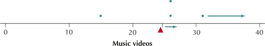 FIGURE 4 As the number of Michael Jackson's videos increases, so does the mean, but not the median or mode.
4 Skewness and Measures of Center
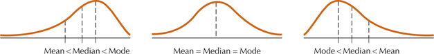
The skewness of a distribution can often tell us something about the relative values of the mean, median, and mode (see Figure 5).
How Skewness Affects the Mean and Median
- For a right-skewed distribution, the mean is larger than the median.
- For a left-skewed distribution, the median is larger than the mean.
- For a symmetric unimodal distribution, the mean, median, and mode are fairly close to each other.
EXAMPLE 7 Mean, median, and skewness
darts
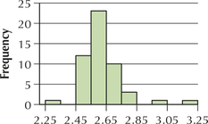
The histogram of the average size of households in the 50 states and the District of Columbia from Example 21 of Chapter 2 (page 74) is reproduced here as Figure 6.
- Based on the skewness of the distribution, state the relative values of the mean, median, and mode.
- Use Minitab to verify your claim in (a).
Solution
- The distribution of average household size is somewhat right-skewed. Thus, from Figure 6, we would expect the mean to be greater than the median, which is greater than the mode.
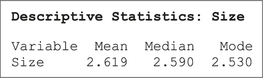
- The Minitab descriptive statistics are shown here. Note that the mean is greater than the median, which is greater than the mode.
NOW YOU CAN DO
Exercises 41–44.

 Can the Financial Experts Beat the Darts?
Recall the contest held by the Wall Street Journal to compare the performance of stock portfolios chosen by financial experts and stocks chosen at random by throwing darts at the Journal stock pages. We will examine the results of 100 such contests in various ways, using the methods we have learned thus far, and will return to examine them further as we acquire more analysis tools. Let's start by reporting the raw result data. The percentage increase or decrease in stock prices was calculated for the portfolios chosen by the professional fnancial advisers and by the randomly thrown darts, and was compared with the percentage net change in the Dow Jones Industrial Average (DJIA).
Remember: It is often helpful to have a “ballpark” estimate of the mean or other statistics as a reality check of your calculations.
Exploratory Data Analysis
Figure 7 shows comparative dotplots of the percentage net change in price for the professionally selected portfolio, the randomly selected darts portfolio, and the DJIA, over the course of the 100 contests. First, estimate the mean of each distribution by choosing the balance point of the data. This balance spot is the mean. For fun, write down your guess for the mean for the professionals so you can see how close you were when we provide the descriptive statistics later. Now compare this with where you would find the balance spot (mean) for the darts dotplot. Which numerical value is larger: the balance spot for the pros or the darts? Just think: you are comparing the mean portfolio performances for the professionals and the darts without using a formula or a calculator. This is exploratory data analysis. You are using graphical methods to compare numerical statistics.
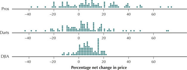
Note: In exploratory data analysis, we use graphical methods to compare numerical statistics.
Hopefully, you discovered that the estimated mean for the pros is greater than the estimated mean for the darts. This is not particularly surprising, is it? Next, find the balance point for the DJIA dotplot. Compare the numerical value for the DJIA balance spot with the mean you found for the dotplot for the pros. Write down your estimate of the means for the DJIA and darts dotplots, so you can see how close you were later. Again, hopefully, you found that the estimated professionals' mean was higher than that of the DJIA. Now, a tougher comparison is to compare the estimated DJIA mean with that of the darts. Which of these two do you think is higher?
Finally, Minitab provides us with the mean percentage net price changes, as shown in Figure 8. Over the course of 100 contests, the mean price for the portfolios chosen by the professional fnancial advisers increased by 10.95%, by 6.793% for the DJIA, and by 4.52% for the random darts portfolio.
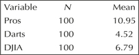
This is evidence in support of the view that fnancial experts can consistently outperform the market.