8.4 Confidence Intervals for the Population Variance and Standard Deviation
OBJECTIVES By the end of this section, I will be able to …
- Describe the properties of the χ2 (chi-square) distribution, and find critical values for the χ2 distribution.
- Construct and interpret confidence intervals for the population variance and standard deviation.
We have seen how confidence intervals can be used to estimate the unknown value of a population mean or a population proportion. However, the variability of a population is also important. As we have learned, less variability is usually better. For example, a tool manufacturer relies on a quality control technician (who has a strong background in statistics) to make sure that the tools the company is making do not vary appreciably from the required specifications. Otherwise, the tools may be too large or too small. Data analysts therefore construct confidence intervals to estimate the unknown value of the population parameters that measure variability: the population variance σ2 and the population standard deviation σ.
We first need to become acquainted with the χ2 (chi-square) distribution, which is used to construct these confidence intervals.
1 Properties of the χ2 (chi-Square) Distribution
The χ2 (pronounced ky-square, to rhyme with “my square”) distribution was discovered in 1875 by the German physicist Friedrich Helmert and further developed in 1900 by the English statistician Karl Pearson. It is a continuous distribution, so the χ2 random variable is continuous.
Just as we did with the normal and t distributions, we can find probabilities associated with values of χ2, and vice versa. Similar to any continuous distribution, probability is represented by area below the curve above an interval. We examine the properties of the χ2 distribution and then learn how to use the χ2 table to find the critical values of the χ2 distribution.
Properties of the χ2 Distribution
- Just as for any continuous random variable, the total area under the χ2 curve equals 1.
- The value of the χ2 random variable is never negative, so the χ2 curve starts at 0. However, it extends indefinitely to the right, with no upper bound.
- Because of the characteristics just described, the χ2 curve is right-skewed.
- There is a different curve for every different degrees of freedom, n−1. As the number of degrees of freedom increases, the χ2 curve begins to look more symmetric (Figure 34).
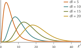 FIGURE 34 Shape of the χ2 distribution for different degrees of freedom.
To construct the confidence intervals in this section, we will need to find the critical values of a χ2 distribution for the given confidence level 100(1−α)%, using either the χ2 table (Table E in the Appendix) or technology. The χ2 table is somewhat similar to the t table (Table D in the Appendix); both tables show the degrees of freedom in the left column. The area to the right of the χ2 critical value is given across the top of the table.
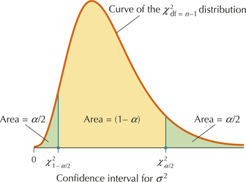
The χ2 distribution is not symmetric, so we cannot construct the confidence interval for σ2 using the “point estimate ± margin of error” method. Instead, the lower bound and upper bound for the confidence interval are determined using two χ2 critical values:
X21−α/2 = the value of the χ2 distribution with area 1−α/2 to its right (Figure 35)
X2α/2 = the value of the χ2 distribution with area 1−α/2 to its right (Figure 35)
For instance, for a 95% confidence interval (1−α)=0.95, α/2=0.025 and 1−α/2=0.975. Thus, χ20.975 represents the value of the χ2 distribution with area 1−α/2=0.975 to the right of the χ2 critical value. The second critical value X20.025 represents the value of the χ2 distribution with area α/2=0.025 to the right of the χ2 critical value.
EXAMPLE 23 Finding the χ2 critical values
Note: If the appropriate degrees of freedom are not given in the χ2 table, the conservative solution is to take the next row with the smaller df.
Find χ2 critical values for a 90% confidence interval, where we have a sample size of size n=10.
Solution
For a 90% confidence interval,
(1−α)=0.90α2=0.102=0.051−α2=1−0.05=0.95
So we are seeking (1) χ20.95, the critical value with area 1−α/2=0.95 to the right of it, and (2) χ20.05, the critical value with area α/2=0.05 to the right of it.
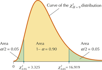
Because n=10, the degrees of freedom is df=n−1=10−1=9. To find χ20.95 for df = 9, go across the top of the χ2 table (Table E in the Appendix) until you see 0.95 (Figure 36). χ20.95 is somewhere in that column. Now go down that column until you see your number of degrees of freedom df = 9. Thus, for df = 9, χ20.95=3.325. For a χ2 distribution with 9 degrees of freedom, there is area = 0.95 to the right of 3.325.
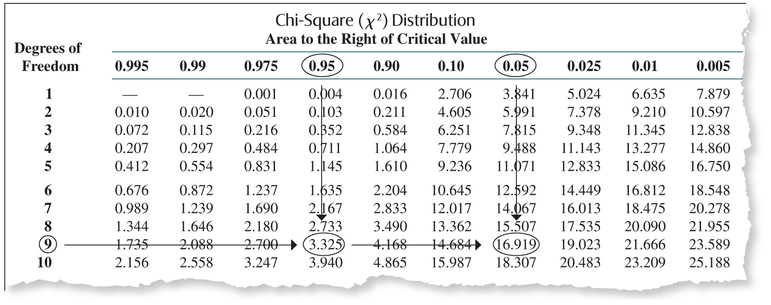
Similarly, χ20.05 is found in the column labeled “0.05” and the row corresponding to df=9. We find that χ20.05=16.919, as shown in Figure 37.
NOW YOU CAN DO
Exercises 9–16.
YOUR TURN#16
Find χ2 critical values for a 95% confidence interval, where we have a sample size of size n=20.
(The solutions are shown in Appendix A.)
2 Constructing Confidence Intervals for the Population Variance and Standard Deviation
We derive the formula for a 100(1−α)% confidence interval for the population variance σ2. Suppose we take a random sample of size n from a normal population with mean μ and standard deviation σ. Then the statistic
χ2=(n−1)s2σ2
follows a χ2 distribution with n−1 degrees of freedom, where s2 represents the sample variance. From Figure 35, we see that 100(1−α)% of the values of χ2 lie between χ21−α/2 and χ2α/2. These values are described as
χ21−α/2<(n−1)s2σ2<χ2α/2
Rearranging this inequality so that σ2 is in the numerator gives us the formula for the 100(1−α)% confidence interval for σ2:
(n−1)s2χ2α/2<σ2<(n−1)s2χ21−α/2
Thus, the lower bound of the confidence interval for σ2 is (n−1)s2χ2α/2, and the upper bound is (n−1)s2χ21−α/2. Taking the square root of each gives us the lower and upper bounds or the confidence interval for σ.
Confidence Interval for the Population Variance σ2
Suppose we take a sample of size n from a normal population with mean μ and standard deviation σ. Then a 100(1−α)% confidence interval for the population variance σ2 is given by
lower bound=(n−1)s2χ2α/2,upper bound=(n−1)s2χ21−α/2
where s2 represents the sample variance and χ21−α/2 and χ2α/2 are the critical values for a χ2 distribution with n−1 degrees of freedom.
Confidence Interval for the Population Standard Deviation σ
A 100(1−α)% confidence interval for the population standard deviation σ is then given by
lower bound=√(n−1)s2χ2α/2,upper bound=√(n−1)s2χ21−α/2
EXAMPLE 24 Constructing confidence intervals for the population variance σ2 and population standard deviation σ

 electricmiles
The accompanying table shows the miles-per-gallon equivalent (MPGe) for fve electric cars, as reported by www.hybridcars.com in 2014. The normal probability plot in Figure 38 indicates that the data are normally distributed.
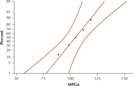
| Electric Vehicle | Mileage (MPGe) |
|---|---|
| Tesla Model S | 89 |
| Nissan Leaf | 99 |
| Ford Focus | 105 |
| Mitsubishi i-MiEV | 112 |
| Chevrolet Spark | 119 |
- Find the critical values χ21−α/2 and χ2α/2 for a confidence interval with a 95% confidence level.
- Construct and interpret a 95% confidence interval for the population variance of electric car MPG.
- Construct and interpret a 95% confidence interval for the population standard deviation of electric car MPG.
electricmiles
Solution
There are n=5 electric cars in our sample, so the degrees of freedom equal n−1=4.
For a 95% confidence interval,
(1−α)=0.95α/2=0.0251−α/2=0.975
From the χ2 table (Table E in the Appendix), therefore,
χ21−α/2=χ20.975=0.484χ2α/2=χ20.025=11.143
Figures 39 through 41 show these results using Excel, Minitab, and JMP.
Figure 42 shows the descriptive statistics for MPGe, as obtained by the TI-83/84. The sample standard deviation is s=11.58447237.
Page 478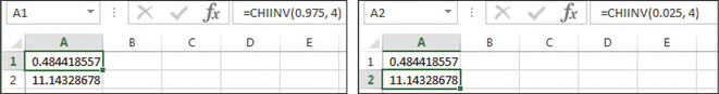 FIGURE 39 Excel results.
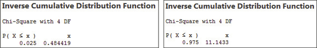 FIGURE 40 Minitab results.
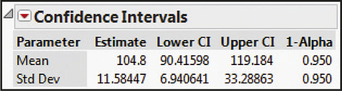
 FIGURE 41 JMP results.
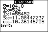 FIGURE 42 TI-83/84 results.
Thus, our 95% confidence interval for σ2 is given by
lower bound=(n−1)s2χ2α/2=(4)11.58447237211.143≈48.1737414≈48.17upper bound=(n−1)s2χ21−α/2=(4)11.5844723720.484≈1109.09091≈1109.09
We are 95% confident that the population variance σ2 lies between 48.17 and 1109.09 miles per gallon squared, that is, (MPG)2. (Recall that the variance is measured in units squared.) It is unclear what miles per gallon squared means, so we prefer to construct a confidence interval for the population standard deviation σ.
- Using the results from part (b),
lower bound=√(n−1)s2χ2α/2=√48.1737414≈6.94073061≈6.94upper bound=√(n−1)s2χ21−α/2=√1109.09091≈33.30301653≈33.3
We are 95% confident that the population standard deviation σ lies between 6.94 and 33.3 miles per gallon. Figure 43 shows the two confidence intervals obtained using Minitab.
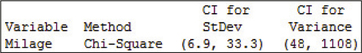
Figure 44 shows the confidence interval for σ obtained using JMP. We are interested in the bottom row, which has the confidence interval for the population standard deviation σ.
NOW YOU CAN DO
Exercises 17–32.