Section 8.2 Exercises
CLARIFYING THE CONCEPTS
Question 8.98
1. Why do we need the t interval? Why can't we always use Z intervals? (pp. 448–449)
8.2.1
In most real-world problems, the population standard deviation σ is unknown, so we can't use the Z interval.
Question 8.99
2. Suppose that σ is known. Should we still use a t interval? (p. 453)
Question 8.100
3. As the sample size gets larger and larger, what happens to the t curve? (p. 450)
8.2.3
The t curve approaches closer and closer to the Z curve.
Question 8.101
4. State the formula for the margin of error for the t interval. (p. 454)
PRACTICING THE TECHNIQUES
 CHECK IT OUT!
| To do | Check out | Topic |
|---|---|---|
| Exercises 5–8 | Example 12 | Finding tα/2 |
| Exercises 9–12 | Example 13 | Checking whether the conditions are met for the t interval for μ |
| Exercises 13–28 | Example 14 | Constructing a t confidence interval for μ |
| Exercises 29–40 | Example 15 | Margin of error |
Question 8.102
5. For the following scenarios, we are taking a random sample from a normal population with σ unknown. Find tα/2.
- Confidence level 90%, sample size 21
- Confidence level 95%, sample size 21
- Confidence level 99%, sample size 21
8.2.5
(a) 1.725 (b) 2.086 (c) 2.845
Question 8.103
6. For the following scenarios we are taking a random sample from a normal population with σ unknown. Find tα/2.
- Confidence level 95%, sample size 11
- Confidence level 95%, sample size 21
- Confidence level 95%, sample size 31
Question 8.104
7. Refer to Exercise 5.
- Describe what happens to the value of tα/2, as the confidence level increases, for a given sample size.
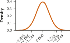
- Draw a sketch of the t curve for sample size n = 21, and explain why the value of tα/2 changes as it does.
8.2.7
(a) For a given sample size, the value of tα/2 increases as the confidence level increases. (b) As the value of tα/2 increases, the confidence interval becomes wider. With a wider confidence interval you can be more confident that your confidence interval contains μ.
Question 8.105
8. Refer to Exercise 6.
- Describe what happens to the value of tα/2, as the sample size increases, for a given confidence level.
- Draw a sketch of the t curve for a confidence level of 95%, and explain why the value of tα/2 changes as it does.
For each of Exercises 9–12, we are taking a random sample from a population with σ unknown. Check whether the conditions are met for constructing the indicated t interval for μ. If not, explain why not.
Question 8.106
9. Confidence level 95%, n = 16, ˉx=250, s = 20
8.2.9
The sample size is not large (n is not ≥30) and we are not told that the population is normal. Therefore, the conditions are not met for the t interval for μ. It is not okay to construct the t interval.
Question 8.107
10. Confidence level 99%, n = 225, ˉx=10, s = 5, normal population
Question 8.108
11. Confidence level 95%, n = 81, ˉx=22, s = 3
8.2.11
We are not told that the population is normal. However, the sample size is large (n is ≥30). Therefore, the conditions are met for the t interval for μ. It is okay to construct the t interval.
Question 8.109
12. Confidence level 90%, n = 64, ˉx=0, s = 8
For the data sets shown in Exercises 13–16, assume the populations are normal, and do the following:
- Calculate ˉx and s.
- Find tα/2.
- Construct and interpret a 95% confidence interval for μ.
Question 8.110
13.
| 4 | 5 | 3 | 5 | 3 |
8.2.13
(a) ˉx=4,s=3 (b) tα/2=2.776 (c) (2.759, 5.241). We are 95% confident that the population mean μ lies between 2.759 and 5.241.
Question 8.111
14.
| 18 | 14 | 16 | 14 | 18 |
Question 8.112
15.
| 10 | 16 | 13 | 16 | 10 |
8.2.15
(a) ˉx=13,s=3 (b) tα/2=2.776 (c) (9.276, 16.724). We are 95% confident that the population mean μ lies between 9.276 and 16.724.
Question 8.113
16.
| 100 | 108 | 104 | 100 | 108 |
For Exercises 17–22, we are taking a random sample from a normal population with σ unknown.
- Find tα/2.
- Confirm that the requirements are met for the t confidence interval for μ.
- Construct the confidence interval for μ with the indicated confidence level.
- Sketch the confidence interval on a number line.
Question 8.114
17. Confidence level 90%, sample size 16, sample mean 10, sample standard deviation 5
8.2.17
(a) tα/2=1.753 (b) We are told that the population is normal. (c) (7.8, 12.2); We are 90% confident that the population mean μ lies between 7.8 and 12.2.
(d)

Question 8.115
18. Confidence level 95%, sample size 16, sample mean 22, sample standard deviation 3
Question 8.116
19. Confidence level 99%, n=9, ˉx=50, s=6
8.2.19
(a) tα/2=3.355 (b) We are told that the population is normal. (c) (43.3, 56.7). We are 99% confident that the population mean μ lies between 43.3 and 56.7.
(d)

Question 8.117
20. Confidence level 95%, n=25, ˉx=0, s=8
Question 8.118
21. Confidence level 95%, n=400, ˉx=−20, s=6
8.2.21
(a) tα/2=1.984 (b) We are told that the population is normal. (c) (−20.6, −19.4). We are 95% confident that the population mean μ lies between −20.6 and −19.4.
(d)

Question 8.119
22. Confidence level 90%, n=100, ˉx=0, s=15
For Exercises 23–28, we are taking a random sample from a population with σ unknown. However, do not assume that the population is normally distributed.
- Find tα/2.
- Confirm that the requirements are met for the t confidence interval for μ.
- Construct the confidence interval for μ with the indicated confidence level.
- Sketch the confidence interval on a number line.
Question 8.120
23. Confidence level 90%, sample size 256, sample mean 100, sample standard deviation 16.
8.2.23
(a) tα/2=1.660 (b) We are not told that the population is normal. However, the sample size is large (n is ≥30). (c) (98.3, 101.7). We are 90% confident that the population mean μ lies between 98.3 and 101.7.
(d)

Question 8.121
24. Confidence level 95%, sample size 100, sample mean 250, sample standard deviation 10.
Question 8.122
25. Confidence level 90%, n=225, ˉx=35, s=5
8.2.25
(a) tα/2=1.660 (b) We are not told that the population is normal. However, the sample size is large (n is ≥30). (c) (34.4, 35.6). We are 90% confident that the population mean μ lies between 34.4 and 35.6.
(d)

Question 8.123
26. Confidence level 99%, n=144, ˉx=42, s=6
Question 8.124
27. Confidence level 95%, n=64, ˉx=−20, s=4
8.2.27
(a) tα/2=2.000 (b) We are not told that the population is normal. However, the sample size is large (n is ≥30). (c) (−21, −19). We are 95% confident that the population mean μ lies between −21 and −19.
(d)

Question 8.125
28. Confidence level 95%, n=400, ˉx=0, s=10
For Exercises 29–40, calculate and interpret the margin of error for the confidence interval from the indicated exercise.
Question 8.126
29. Exercise 17
8.2.29
E=2.2. We can estimate the population mean μ to within 2.2 with 90% confidence.
Question 8.127
30. Exercise 18
Question 8.128
31. Exercise 19
8.2.31
E=6.7. We can estimate the population mean μ to within 6.7 with 99% confidence.
Question 8.129
32. Exercise 20
Question 8.130
33. Exercise 21
8.2.33
E=0.6. We can estimate the population mean μ to within 0.6 with 95% confidence.
Question 8.131
34. Exercise 22
Question 8.132
35. Exercise 23
8.2.35
E=1.7. We can estimate the population mean μ to within 1.7 with 90% confidence.
Question 8.133
36. Exercise 24
Question 8.134
37. Exercise 25
8.2.37
E=0.6. We can estimate the population mean μ to within 0.6 with 90% confidence.
Question 8.135
38. Exercise 26
Question 8.136
39. Exercise 27
8.2.39
E=1. We can estimate the population mean μ to within 1 with 95% confidence.
Question 8.137
40. Exercise 28
APPLYING THE CONCEPTS
Question 8.138
41. Hospital Length of Stay. The U.S. Agency for Healthcare Research and Quality reports that the mean length of stay in the hospital for patients suffering from acute myocardial infarction (heart attack) was 4.8 days. Suppose a sample of 31 heart attack patients had a mean length of stay of 4.8 days, with a sample standard deviation of 3 days. Do the following:
- State how the conditions for the t interval for μ are met.
- Find tα/2 for a confidence interval with 95% confidence.
- Construct and interpret a 95% confidence interval for the population mean length of stay for all heart attack victims.
8.2.41
(a) We are not told that the population is normal. However, the sample size is large (n is ≥30). (b) tα/2=2.042 (c) (3.7, 5.9). We are 95% confident that μ, the population mean length of stay in hospital for all heart attack victims, lies between 3.7 days and 5.9 days.
Question 8.139
42. Student loans. The Pew Research Center (www.pewresearch.org) reports that the mean student loan amount in 2010 was $26,682. Suppose a sample of 41 students had a sample mean loan amount of $26,682 and a sample standard deviation student loan amount of $20,000. Do the following:
- State how the conditions for the t interval for μ are met.
- Find tα/2 for a confidence interval with 90% confidence.
- Construct and interpret a 90% confidence interval for the population mean student loan amount.
Question 8.140
43. Consumer Sentiment. The University of Michigan Surveys of Consumers found that the mean index of consumer sentiment for December 2013 was 82.5. Suppose this result was based on a sample of size 100, which had a standard deviation of 10.
- State how the conditions for the t interval for μ are met.
- Find tα/2 for a confidence interval with 95% confidence.
- Construct and interpret a 95% confidence interval for the population mean consumer sentiment.
8.2.43
(a) We are not told that the population is normal. However, the sample size is large (n is ≥30). (b) tα/2=1.987 (c) (80.5, 84.5). We are 95% confident that μ, the population mean consumer sentiment for all consumers, lies between 80.5 and 84.5.
Question 8.141
44. Teachers' Salaries. The Digest of Educational Statistics reported that the mean salary for teachers in 2012 was $56,410. Assume that the sample size was 101 and the sample standard deviation was $15,000.
- State how the conditions for the t interval for μ are met.
- Find tα/2 for a confidence interval with 90% confidence.
- Construct and interpret a 90% confidence interval for the population mean teacher salary.
Question 8.142
45. Hospital Length of Stay. Refer to Exercise 41.
- Calculate and interpret the margin of error.
- If the sample size is increased to 400, describe what will happen to the margin of error.
8.2.45
(a) E=1.1 days. We can estimate the population mean length of stay in hospital of all heart attack victims to within 1.1 days with 95% confidence. (b) It decreases.
Question 8.143
46. Student Loans. Refer to Exercise 42.
- Calculate and interpret the margin of error.
- If the sample size is increased to 100, describe what will happen to the margin of error.
Question 8.144
47. Consumer Sentiment. Refer to Exercise 43.
- Compute the margin of error and interpret it.
- Describe two ways of reducing this margin of error. Which method is more desirable, and why?
8.2.47
(a) E=2. We can estimate the population mean consumer sentiment for all consumers to within 2 with 95% confidence. (b) Decrease the confidence level or increase the sample size; Increase the sample size; The only way to have both high confidence and a tight interval is to boost the sample size.
Question 8.145
48. Teachers' Salaries. Refer to Exercise 44.
- Compute the margin of error and interpret it.
- Describe two ways of reducing this margin of error. Which method is more desirable, and why?
For Exercises 49–56, software output for t confidence intervals for μ are provided. Assume the conditions are met. For each, examine the indicated software output, and do the following:
- Report the confidence interval in the form “(lower bound, upper bound).”
- Interpret the confidence interval.
- Calculate the margin of error for the confidence interval.
- Interpret the margin of error.
Question 8.146
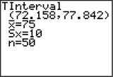
49. Exam Scores. TI-83/84 output, where μ represents the population mean exam score. Confidence level is 95%.
8.2.49
(a) (72.2, 77.8) (b) We are 95% confident that μ, the population mean exam score for all exam takers, lies between 72.2 and 77.8. (c) 2.8 (d) We can estimate the population mean exam score for all exam takers to within 2.8 with 95% confidence.
Question 8.147
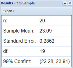
50. Clothing Store Sales. Minitab output, where μ represents the population mean total net sales for a clothing store.

Question 8.148
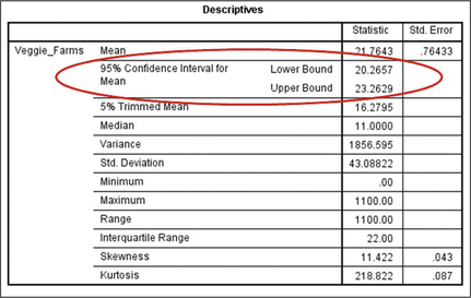
51. Vegetable Farms. SPSS output, where μ represents the population mean number of vegetable farms per county, nationwide.
8.2.51
(a) (20.3, 23.3) (b) We are 95% confident that μ, the population mean number of vegetable farms per county for all counties nationwide, lies between 20.3 vegetable farms per county and 23.3 vegetable farms per county. (c) 1.5 vegetable farms per county (d) We can estimate the population mean number of vegetable farms per county for all counties nationwide to within 1.5 vegetable farms per county with 95% confidence.
Question 8.149
52. Grocery Stores. JMP output, where μ represents the population mean number of grocery stores per county, nationwide.

Question 8.150
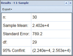
53. Small Businesses. Crunchit! Output, where μ represents the population mean number of small businesses per city, nationwide. Note: The notation “e+4” means to move the decimal place four places to the right. So, “2.240e+4,” moving the decimal place four places to the right, gives us 22,400.
8.2.53
(a) (22,400, 25,630) (b) We are 95% confident that μ, the population mean number of small businesses per city for all cities nationwide, lies between 22,400 small businesses per city and 25,630 small businesses per city. (c) 1615 small businesses per city (d) We can estimate the population mean number of small businesses per city for all cities nationwide to within 1615 small businesses per city with 95% confidence.
Question 8.151
54. Protein Content in Breakfast Cereal. For the SPSS output, μ represents the population mean amount of protein, in grams, for all breakfast cereals.

Question 8.152
55. Sugar Content in Breakfast Cereal. For the JMP output, μ represents the population mean amount of sugars, in grams, for all breakfast cereals.

8.2.55
(a) (6.08, 7.77) (b) We are 90% confident that μ, the population mean amount of sugar for all breakfast cereals, lies between 6.08 grams and 7.77 grams. (c) 0.84 gram (d) We can estimate the population amount of sugar for all breakfast cereals to within 0.84 gram with 90% confidence.
Question 8.153
56. Fourth-Graders' Feet. For the CrunchIt! Output, μ represents the population mean length of fourth-graders' feet, in cm.
Question 8.154
carbon
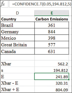
57. Carbon Emissions. The Excel output shows the carbon emissions (in millions of tons) from consumption of fossil fuels for a random sample of five nations.12 The sample mean (using the function “average”) and the sample standard deviation (using the function “stdev”) are also given. The highlighted cell is the margin of error given by the function CONFIDENCE.T, which needs the following values: 1−α, s, and n. Below, the normal probability plot is given.
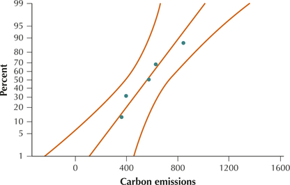
- Check the normality assumption.
- Use the Excel output to report and interpret a 95% t confidence interval for the population mean carbon emissions.
- Use the Excel output to report and interpret the margin of error for the confidence interval in part (b).
- Explain two ways we could decrease the margin of error. Which method is preferable, and why?
8.2.57
(a) Acceptable normality (b) (320.31, 804.09). We are 95% confident that μ, the population mean carbon emissions for all nations, lies between 320.31 million tons and 804.09 million tons. (c) E=241.89 million tons; We can estimate the population mean carbon emissions for all nations to within 241.89 million tons with 95% confidence. (d) Decrease the confidence level or increase the sample size. Increase the sample size. The only way to have both high confidence and a tight interval is to boost the sample size.
Question 8.155
deepwaterclean
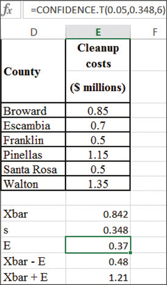
58. Deepwater Horizon Cleanup Costs. The Excel output shows the amount of money disbursed by BP to a random sample of six Florida counties for cleanup of the Deepwater Horizon oil spill, in millions of dollars.13 The functions used to provide the confidence interval are similar to those in Exercise 57. The normal probability plot is also given.
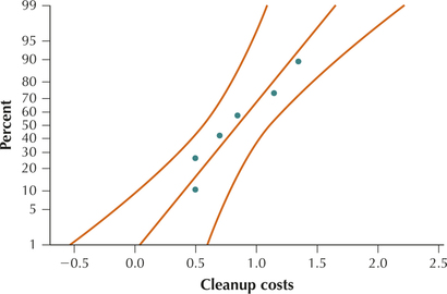
- Check the normality assumption.
- Use the Excel output to report and interpret a 95% t confidence interval for the population mean cleanup cost.
- Use the Excel output to report and interpret the margin of error for the confidence interval in part (b).
- Explain two ways we could decrease the margin of error. Which method is preferable, and why?
Question 8.156
wiisales
59. Wii Game Sales. The following table represents the number of units sold (in 1000s) in the United States for the week ending March 26, 2011, for a random sample of 8 Wii games.14 The normal probability plot is given.
| Game | Units (1000s) |
Game | Units (1000s) |
|---|---|---|---|
| Wii Sports Resort | 65 | Zumba Fitness | 56 |
| Super Mario All Stars |
40 | Wii Fit Plus | 36 |
| Just Dance 2 | 74 | Michael Jackson | 42 |
| New Super Mario Brothers |
16 | Lego Star Wars | 110 |
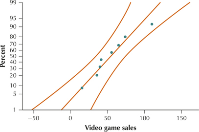
- Confirm that the normality condition is met.
- Construct and interpret a 95% confidence interval for the population mean number of units sold.
- Calculate and interpret the margin of error.
- How could we decrease the margin of error of our confidence interval without decreasing the confidence level?
8.2.59
(a) Acceptable normality (b) (31, 79). We are 95% confident that μ, the population mean number of Wii game units sold per week for all weeks, lies between 31 thousand units and 79 thousand units. (c) E=24 thousand units. We can estimate the population mean number of Wii game units sold per week for all weeks to within 24 thousand units with 95% confidence. (d) Decrease the confidence level or increase the sample size. Increase the sample size. The only way to have both high confidence and a tight interval is to boost the sample size.
Question 8.157
georgiarain
60. A Rainy Month in Georgia? The following table represents the total rainfall (in inches) for the month of February 2011 for a random sample of 10 locations in Georgia.15
| Location | Rainfall (inches) |
Location | Rainfall (inches) |
|---|---|---|---|
| Athens | 4.72 | Atlanta | 4.25 |
| Augusta | 4.31 | Cartersville | 3.03 |
| Dekalb | 2.96 | Fulton | 4.36 |
| Gainesville | 4.06 | Lafayette | 3.75 |
| Marietta | 3.20 | Rome | 3.26 |
- Use technology to construct a normal probability plot to confirm that the data exhibit acceptable normality.
- Construct and interpret a 90% confidence interval for the population mean rainfall in inches.
- Calculate and interpret the margin of error.
- How could we decrease the margin of error of our confidence interval without decreasing the confidence level?
Question 8.158
electricmiles
61. Electric Cars. The accompanying table shows the miles-per-gallon equivalent (MPGe) for five electric cars, as reported by www.hybridcars.com in 2014.
| Electric Vehicle | MPGe |
|---|---|
| Tesla Model S | 89 |
| Nissan Leaf | 99 |
| Ford Focus | 105 |
| Mitsubishi i-MiEV | 112 |
| Chevrolet Spark | 119 |
- Use technology to construct a normal probability plot of MPGe. Confirm that the distribution is normal.
- Find tα/2 for a confidence interval with 90% confidence.
- Compute and interpret the margin of error E for a confidence interval with 90% confidence.
- Construct and interpret a 90% confidence interval (t interval) for the population mean mileage.
8.2.61
(a)
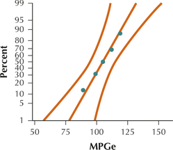
Acceptable normality. (b) tα/2=2.132 (c) E=11.0 MPGe. We can estimate the population mean mileage to within 11.0 MPGe with 90% confidence.
(d) (93.8, 115.8). We are 90% confident that μ, the population mean mileage, lies between 93.8 MPGe and 115.8 MPGe.
Question 8.159
cerealcalories
62. Calories in Breakfast Cereals. What is the mean number of calories in a bowl of breakfast cereal? A random sample of six well-known breakfast cereals yielded the following calorie data:
| Cereal | Calories |
|---|---|
| Apple Jacks | 110 |
| Cocoa Puffs | 110 |
| Mueslix | 160 |
| Cheerios | 110 |
| Corn Flakes | 100 |
| Shredded Wheat | 80 |
- Use technology to construct a normal probability plot of the number of calories.
- Is there evidence that the distribution is not normal?
- Can we proceed to construct a t interval? Why or why not?
Question 8.160
commutedist
63. Commuting Distances. A university is trying to attract more commuting students from the local community. As part of the research into the modes of transportation students use to commute to the university, a survey was conducted asking how far commuting students commuted from home to school each day. A random sample of 30 students provided the distances (in miles) shown.
| 14 | 10 | 14 | 12 | 12 | 11 | 5 | 6 | 9 | 14 | 9 | 9 | 4 | 7 | 15 |
| 9 | 7 | 7 | 12 | 10 | 15 | 10 | 6 | 11 | 9 | 11 | 10 | 11 | 7 | 12 |
- Find tα/2 for a confidence interval with 90% confidence.
- Compute and interpret the margin of error for a confidence interval with 90% confidence.
- Construct and interpret a 90% t confidence interval for the population mean commuting distance.
8.2.63
(a) tα/2=1.699 (b) E=0.9 mile. We can estimate the population mean commuting distance to within 0.9 mile with 90% confidence. (c) (9.0, 10.8). We are 90% confident that μ, the population mean commuting distance, lies between 9.0 miles and 10.8 miles.
Question 8.161
 64. Refer to the previous exercise. What if we increased the sample size to some unspecified value but everything else stayed the same. Describe what, if anything, would happen to each of the following measures and why:
- tα/2
- Margin of error E
- Width of the confidence interval
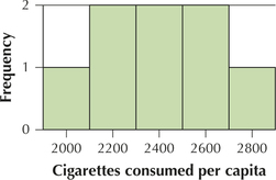
Cigarette Consumption. Use the following information for Exercises 65–67. Health officials are interested in estimating the population mean number of cigarettes smoked annually per capita in order to evaluate the efficacy of their antismoking campaign. A random sample of eight U.S. counties yielded the following numbers of cigarettes smoked per capita: 2206, 2391, 2540, 2116, 2010, 2791, 2392, 2692.
Question 8.162
65. Evaluate the normality assumption using the accompanying histogram. Is it appropriate to construct a t interval using this data set? Why or why not? What is it about the histogram that tells you one way or the other?
8.2.65
The graph is symmetric about the middle value with the values with the highest frequency in the middle. This indicates that the normality assumption is valid. Since the normality assumption appears to be valid and σ is unknown, Case 1 applies, so we can use the t interval.
Question 8.163
66. Compute and interpret the margin of error E for a confidence interval with 90% confidence. What is the meaning of this number?
Question 8.164
67. Construct and interpret a 90% confidence interval for the population mean number of cigarettes smoked per capita.
8.2.67
(2208, 2576). We are 90% confident that μ, the population mean number of cigarettes smoked per capita, lies between 2208 cigarettes and 2576 cigarettes.
Question 8.165
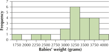
68. Baby Weights. A random sample of 20 babies born in Brisbane (Australia) Hospital had the histogram of the babies' weights shown here. The sample mean is 3227 grams, and the sample standard deviation is 560 grams. Discuss the normality of the data. Do the data appear acceptably normal? Is it appropriate to apply the t interval or not? Explain why or why not.
BRINGING IT ALL TOGETHER
 Chapter 8 Case Study: Motor Vehicle Fuel Efficiency.
Use the following information for Exercises 69–74. The Environmental Protection Agency calculates the estimated annual fuel cost for motor vehicles, with the resulting data provided in the variable annual fuel cost of the Chapter 8 Case Study data set Fuel Efficiency. A sample of the annual fuel cost is provided for 12 vehicles.
| Annual fuel cost | |||
|---|---|---|---|
| 1750 | 2500 | 2400 | 2350 |
| 2150 | 3100 | 2950 | 2500 |
| 2550 | 2750 | 2300 | 2800 |
Question 8.166
69. Construct a normal probability plot of the data (see pages 381–384). Evaluate the normality assumption using the accompanying histogram. Is it appropriate to construct a t interval using this data set? Why or why not?
8.2.69
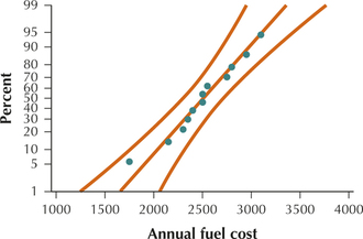
Acceptable normality.
Question 8.167
70. Find the point estimate of μ, the population mean annual fuel cost.
Question 8.168
71. Compute the sample standard deviation s.
8.2.71
s=$366.1
Question 8.169
72. Find tα/2 for a confidence interval with 90% confidence.
Question 8.170
73. Construct and interpret a 90% confidence interval for the population mean annual fuel cost.
8.2.73
(2318.2, 2697.8). We are 90% confident that μ, the population mean annual fuel cost, lies between $2318.2 and $2697.8.
Question 8.171
74. Compute and interpret the margin of error E for a confidence interval with 90% confidence. What is the meaning of this number?
WORKING WITH LARGE DATA SETS
 Chapter 8 Case Study: Motor Vehicle Fuel Efficiency.
Open the Chapter 8 Case Study data set Fuel Efficiency. Here, we will examine confidence intervals for the population mean amount of carbon dioxide generated by motor vehicles in city driving. We will then see whether these confidence intervals succeeded in capturing the population mean amount of carbon dioxide. Use technology to do the following:  fueleffciency
Question 8.172
75. Obtain a random sample of size 100 from the data set.
8.2.75
Answers will vary.
Question 8.173
76. Suppose we are interested in constructing a 95% t interval for the population mean amount of carbon dioxide generated by these vehicles in city driving (the variable city CO2), using our sample from the previous exercise. Do we need to check for normality?
Question 8.174
77. Construct and interpret a 90% t interval for the population mean amount of city CO2.
8.2.77
Answers will vary.
Question 8.175
78. Did your interval in Exercise 77 capture the population mean? Check by finding the mean city CO2 of all the vehicles.
Question 8.176
79. Generate a second sample of size 100 from the data set. Construct a second 90% t interval for the population mean amount of city CO2. Did this confidence interval capture the population mean?
8.2.79
Answers will vary.
Question 8.177
80. If we keep on obtaining new samples all day long, about what proportion of the 90% confidence intervals will capture the population mean?