4.2 4.1 Linear Programming and Mixture Problems: Combining Resources to Maximize Profit
Here, we learn about linear programming, a management science technique that helps a business allocate its resources. Whether those resources are at hand or can be purchased, the goal is to decide on a particular mix of products that will maximize profit or that will operate in ways that cut costs. For example, a large medical center needs to stock resources such as bandages, syringes, and alcohol wipes, as well as have different kinds of laborers, toilet paper, and paper towels available when needed.
Linear Programming DEFINITION
Linear programming is a tool for maximizing or minimizing a quantity, typically a profit or a cost, subject to a set of constraints.
The technique is so powerful that it is estimated that much more computer time is used solving linear programming types of problems than for any other purpose for which business managers and decision makers use computers.
Linear programming is an example of “new” mathematics. It came into being, along with many other management science techniques, during and shortly after World War II, in the 1940s. It is quite young as intellectual ideas go. Yet, during its short history, linear programming has changed the way businesses and governments make decisions, from ‘"seat-of-the-pants” methods based on guesswork and intuition to using an algorithm based on available data and guaranteed to produce an optimal decision.
Linear programming is but one operations research tool belonging to a family of tools known as mathematical programming. Another such tool is integer programming. The difference between linear programming and integer programming is that for linear programming, the quantities being studied can take on values such as π=3.14159… or 718; in integer programming, the values are confined to whole numbers such as 8, 50, or 1,102,362. Whole numbers are conceptually easier than the broader group consisting of all numbers that can be represented by decimals (1.32, 1.455555…), yet integerprogramming problems have proved much harder to solve.
In the discussions that follow, we often describe “relaxed” versions of integer-programming problems as linear-programming problems. For example, it would make no sense to produce 3.24 dolls to sell. So, strictly speaking, we must find an optimum whole number of dolls to produce. If we are ‘lucky,” the linear-programming problem associated with an integer-programming problem has an integer solution. In this case, we have also found the correct answer to the integer-programming problem. Some other examples that fall into this category are discussed below.
Linear programming has saved businesses and governments billions of dollars. Of all the management science techniques presented in this book, linear programming is far and away the most frequently used. It can be applied in a variety of situations, in addition to the one we study in this chapter. Some of the problems studied in Chapters 1, 2, and 3—for example, the traveling salesman (TSP) and scheduling problems—can be viewed as linear-programming problems. Linear programming is an excellent example of a mathematical technique useful for solving many different kinds of problems that at first do not seem to be similar problems at all. It has been suggested that without linear programming, management science would never have been born as a special branch of knowledge.
Next, we study how to use linear programming to solve a special kind of problem—a mixture problem. Realistic versions of such problems would be much more involved. Our discussion is designed to give you the flavor of what is actually done. Realistic examples of what follows are commonly used in the manufacture of different kinds of breads from the grain flours available, and in the making of different kinds of sausages from meats such as beef and pork.
Mixture Problem DEFINITION
In a mixture problem, limited resources are combined into products so that the profit from selling those products is as large as possible—a maximum.
Mixture problems are widespread because nearly every product in our economy is created by combining resources. A typical example would be how different kinds of aviation fuel are manufactured using different kinds of crude oil.
Let’s analyze small versions of the kinds of problems that might confront a toy or a beverage manufacturer. Both manufacturers can sell many different products on which each company can make a profit. There could be dozens of possible products and many resources. A manufacturer must periodically look at the quantities and prices of resources and then determine which products should be produced in which quantities in order to gain the greatest, or optimum, profit (see Spotlight 4.1). This is an enormous task that usually requires a computer to solve.
What does it mean to find a solution to a linear-programming mixture problem? A solution to a mixture problem is a production policy that tells us how many units of each product to make.
Optimal Production Policy DEFINITION
An optimal production policy has two properties:
- It is possible; that is, it does not violate any of the limitations under which the manufacturer operates, such as availability of resources.
- It gives the maximum profit.
Common Features of Mixture Problems
Although our first mixture problem (Example 1) has only two products and one resource, it does contain the essential features that are common to all mixture problems:
- Resources. Definite resources are available in limited, known quantities for the time period in question. The resource in Example 1 is containers of plastic.
- Products. Definite products can be made by combining, or mixing, the resources. In Example 1, the products are skateboards and dolls.
Case Studies in Linear Programming 4.1
4.1
Linear programming is not limited to mixture problems. Here are two case studies that do not involve mixture problems, yet applying linear-programming techniques produced impressive savings:
- The Exxon Corporation spends several million dollars per day running refineries in the United States. Because running a refinery takes a lot of energy, energy-saving measures can have a large effect. Managers at Exxon’s Baton Rouge plant had over 600 energy-saving projects under consideration. They couldn’t implement them all because some conflicted with others, and there were so many ways of making a selection from the 600 that it was impossible to evaluate all selections individually.
Exxon used linear programming to select an optimal configuration of about 200 projects, resulting in millions of dollars in savings.
- Edwards Lifesciences uses heart valves from pigs to produce artificial heart valves for human beings. Pig heart valves come in different sizes. Shipments of pig heart valves often contain too many of some sizes and too few of others. However, each supplier tends to ship roughly the same imbalance of valve sizes in every order, so the company can expect consistently different imbalances from the different suppliers. Thus, if they order shipments from all the suppliers, the imbalances could cancel each other out in a fairly predictable way. The amount of cancellation will depend on the sizes of the individual shipments. Unfortunately, there are too many combinations of shipment sizes to consider all combinations individually.
Edwards Lifesciences used linear programming to figure out which combination of shipment sizes would give the best cancellation effect. This reduced the company’s annual cost by $1.5 million.
- Recipes. A recipe for each product specifies how many units of each resource are needed to make one unit of that product. Each skateboard in Example + uses five units of plastic, and each doll uses two units.
- Profits. Each product earns a known profit per unit. (We assume that every unit produced can be sold. More complicated mathematical models, which we will not discuss here, are needed if we want to consider the possibility of items being produced but not sold.)
- Objective. The objective in a mixture problem is to find how much of each product to make so as to maximize the profit without exceeding any of the resource limitations.
The examples we show are not designed to be realistic. Rather, our goal is to demonstrate how ideas whose roots are in basic algebra and geometry can solve, when scaled up to realistic versions, problems that save Americans much time and money and make our government and American businesses more efficient.
EXAMPLE 1![]() Making Skateboards and Dolls
Making Skateboards and Dolls
A toy manufacturer can manufacture only skateboards, only dolls, or some mixture of skateboards and dolls. Skateboards require 5 units of plastic and can be sold for a profit of $1, while dolls require 2 units of plastic and can be sold for a $0.55 profit. If 60 units of plastic are available, what numbers of skateboards and/or dolls should be manufactured for the company to maximize its profit?
Attacking this and other mixture problems requires carrying out a series of steps that determine the essence of the problem.
As a first step, we need to construct a mathematical model to take the “verbal” information that we have been given and display it in a form that makes it easier to convert into the mathematics necessary to solve the problem. This is done by making a mixture chart for the information we are given (see Figure 4.1).
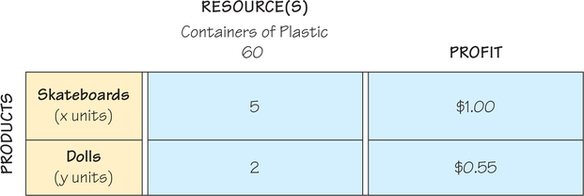
In the rows of this chart, we display the products we want to make, and in the column of the chart, we display the resources and the profit margin information that is available. In this case, we have two products, so we have two rows. We have one resource, which accounts for there being one column.
The other column is reserved for profit information. Since this information is used in a somewhat different way from the information about the resources, we will separate the resource column(s) from the profit column by a double bar.
Because we do not know the number of skateboards the company should make, we will use a letter x to represent the unknown number of skateboard units that the company might manufacture. Similarly, y will represent the number of dolls that the company might manufacture. We enter these letters as part of the labels of the rows of our table.
We can now enter the numbers about resources in the columns based on the information we have been given. in this case, there is one resource: plastic. Thus, for the 5 units of plastic needed for a skateboard, we record a 5 in the skateboards row and the containers of plastic column. Similarly, we enter a 2 in the second row and first column because dolls require 2 units of plastic each. Because we have 60 units of plastic available, we display this fact by placing the number 60 at the top of this column. We complete the table with the information about profit. We enter $1 in the skateboards row and profit column and $0.55 in the dolls row and profit column.
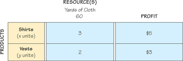
EXAMPLE 2![]() Making a Mixture Chart
Making a Mixture Chart
Make a mixture chart to display (model) this situation: A clothing manufacturer has 60 yards of cloth available to make shirts and decorated vests. Each shirt requires 3 yards of cloth and provides a profit of $5. Each vest requires 2 yards of cloth and provides a profit of $3. A mixture chart is shown in Figure 4.2.
Translating Mixture Charts into Mathematical Form
Consider again the mixture chart in Figure 4.1. What can we say about the numbers of skateboards and dolls that might be manufactured? Clearly, we cannot make negative numbers of skateboards or dolls. Because we are using the letter x to represent the number of skateboards we plan to make, we can write down the algebraic expression that x≥0. Here, we are using the standard symbol ≥ for “greater than or equal to.”
Algebraic expressions that involve the symbol ≥ or its companion symbols ≤ (less than or equal to), > (greater than), and < (less than) are known as inequalities. We can also write down an inequality for the y number of dolls we plan to make, based on the fact that we cannot make a negative number of dolls. Thus, we must have y≥0. We will use the phrase minimum constraints for these two inequalities, x≥0 and y≥0, which mean that we cannot manufacture negative numbers of objects.
However, we also have only a limited number of units of plastic available. How can we represent this information? Consulting the mixture table, we see that we need 5 units of plastic for every skateboard we make. Thus, we will need 5x (5 times x) units of plastic for the x skateboards we make. Similarly, we will need 2y (2 times y) units of plastic for the y dolls we make. Hence we will need 5x+2y units of plastic for the mixture of skateboards and dolls we make. We added the 5x and 2y because we need to find the total plastic used when we make a mixture of skateboards and dolls.
Reading from the table, we see that we are limited by having only 60 units of plastic. So we can express the resource constraint imposed by the limited number of units of plastic by writing that 5x+2y≥60. Here, we use the symbol for less than or equal to, ≤, to express the fact that we cannot use more than the amount of plastic we have available.
Notice that all the numbers in this inequality can be obtained from a column of the mixture chart. One of the reasons that we construct a mixture chart is that it helps speed up the conversion of the information about the problem we wish to solve into inequalities. The setup phase of a realistic linear programming problem, constructing the mathematical model of a manufacturing situation, is often the hardest and most complex step in getting an answer.
In addition to the resource inequalities (of which realistic problems will often have hundreds), there is one additional algebraic expression, this time an equality, that the mixture table allows us to create. Using the mixture table, we can compute the profit that will be produced when we manufacture different mixtures. For each skateboard, we make a profit of $1, so if x skateboards are made, the profit is 1X (1 times x). For each doll made, the profit is $0.55. So if y dolls are made, the profit is 0.55y (0.55 times y). Denoting by P the total profit from making x skateboards and y dolls, we get the equation
P=1x+0.55y

Linear Equations in Two Variables
Note that unlike the situation for the resources where we got an inequality, here we get an expression for what the profit will be as we vary the numbers of skateboards and dolls manufactured. Our goal is to find which values of x and y (skateboards and dolls) make this profit as large as possible.
EXAMPLE 3![]() Revisiting Our Clothing Manufacturer
Revisiting Our Clothing Manufacturer
We can also translate the information in the mixture chart shown in Figure 4.2 into inequalities and an equation for expressing the profit in terms of how many shirts and vests are produced. Using the first column of the mixture chart and the fact that only 60 units of cloth are available, we can write
3x+2y≤60
And using the last column, we get the following expression for the profit P:
P=5x+3y
Now that we have the information from the original problems represented in mathematical terms, we will return our attention to finding a solution to the problems.
Finding the best (largest profit) mixture of skateboards and/or dolls to make can be carried out in two phases.
- Determine those mixtures of skateboards and/or dolls that can be manufactured subject to the limited resources that are available. This step involves finding the feasible set for the mixture problem.
Feasible Set or Feasible Region DEFINITION
The feasible set, also called the feasible region, for a linear-programming problem is the collection of all physically possible solution choices that can be made.
We can use a geometric diagram such as the one in Figure 4.3 to help us understand the feasible set of options that the manufacturer of skateboards and dolls has available. The geometric diagram we draw will have as many “dimensions” as there are products being manufactured. We have two products represented by the variables x and y, so we use a two-dimensional picture. Even diagrams involving three variables are hard to draw and visualize. Though these diagrams helped with developing algorithms for solving mixture problems, they are of little practical use for realistic problems.
- Determine how to pick out, from the feasible set, the mixture (or mixtures) that gives rise to the largest profit.
Representing the Feasible Region with a Picture
After we have constructed inequalities using a mixture chart or have the inequalities that must be obeyed for a more general linear-programming problem, we can draw a helpful picture to visualize the choices to be made in solving the problem. This picture will show in a convenient way the different choices that are available in solving the linear-programming problem at hand. To get the picture that will help us, we need to draw graphs of the inequalities associated with the linear-programming problem.
To draw the graph of an inequality, let’s first review how to draw the graph of the equation of a straight line. Remember that two points can be used to uniquely determine a straight line. Let’s use the equation associated with the less-than-or- equal-to inequality
Linear Inequalities in Two Variables
5x+2y≤60
namely,
5x+2y=60
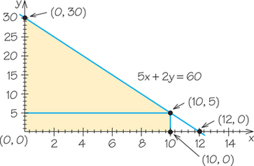
There are two points that are easy to find on this line: the x- and y-intercepts. When x=0, this gives rise to one point on the line, and when y=0, we can find another point. (See Figure 4.3.) When x=0, if we substitute this value in the equation 5x+2y=60, we get 5(0)+2y=60. Solving this equation, we discover that y=30. Similarly, if we substitute y=0 in the equation 5x+2y=60, we get 5x+2(0)=60, from which we conclude that x=12. We now have two points (0, 30) and (12, 0) that lie on the line 5x+2y=60.
We are using the usual convention that when we write a pair such as (3, 10), we are describing a point that has x=3 and y=10. We always list the x-value (x-coordinate) first in such a pair and the y-value (y-coordinate) second. Furthermore, when a point (x, y) is represented in a diagram, larger values of x are shown farther to the right (east) and larger values of y are shown farther up (north).
Using the two points we found on the line 5x+2y=60, we can draw the graph shown in Figure 4.3a, where we have also displayed the point (3, 10). How do we know that (3, 10) is not on the line? We can see this by replacing x by 3 and y by 10 in the equation 5x+2y=60, getting 5(3) + 2(10)=15 + 20=35. To have been on the line, we would have to have had the value 60. Furthermore, we know that the point (3, 10) is below the line 5x+2y=60 because when x=3, and we replace x by this value in the equation 5x+2y=60, we get 5(3)+2y=60, which means that y=45/2. Since 45/2 is greater than 10, the y-value for the point (3, 10), we conclude that (3, 10) is below the line.
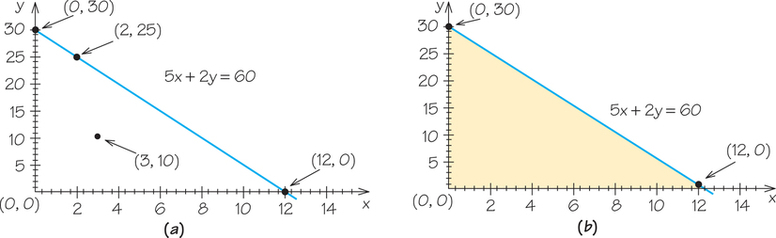
Now that we know what the graph of the equation 5x+2y=60 looks like, we can think through where points (x,y) that satisfy 5x+2y<60 are located. The points that are either on the line 5x+2y=60 or satisfy 5x+2y<60 will satisfy 5x+2y≤60.
Any line, for example, 5x+2y=60, divides the xy-plane into three parts: those points on the line and the points in one of two half-planes. In one of these halfplanes, we have the points for which 5x+2y<60, and in the other, we have the points for which 5x+2y>60. How can we tell which of the two half-planes is above the line 5x+2y=60 and which is below?
The key is the use of a test point (x,y) that is not on the line and whose half-planes we wish to distinguish. We saw above that (3, 10) is not on the line 5x+2y=60 and is below the line. This enables us to see that the half-plane for which 5x+2y<60 consists of the points below the line 5x+2y=60.
To complete the drawing of the points that are feasible for the skateboard and dolls manufacturing problem, we also have to know which points satisfy the constraints that state that the number of skateboards produced x cannot be negative (x≥0) and the number of dolls produced y cannot be negative (y≥0). Each of these inequalities corresponds to a half-plane, and we can again test which of the half-planes associated with the line x=0 is determined by x≥0.
This can be done using the point (3, 10) as a test point again. Because x=3 is greater than 0, x≥0 determines the half-plane to the right of the line x=0 (the y-axis). Similarly, using the point (3, 10), we see that because y=10 is greater than 0, y≥0 determines the half-plane above the line y=0 (the x-axis).
Putting this information together leads us to the conclusion that the collection of points (x,y) that meets the three inequalities involved (x≥0, y≥0, 5x+2y≤60) corresponds to the shaded region in Figure 4.3b. Remember that when graphing equations, lines with equations like x=2 are vertical lines, whereas those like y=4 are horizontal lines.
Note that since the minimality conditions are always present in the kind of linear-programming problems we are dealing with, the points that are feasible for these problems are always in the upper right region (quadrant) that is created by the x-axis and y-axis. Next, we draw the feasible region for the clothing manufacturing problem.
EXAMPLE 4![]() Drawing a Feasible Region
Drawing a Feasible Region
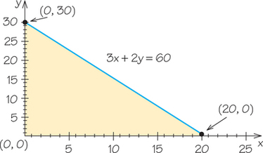
In the earlier clothing manufacturer example, we developed a resource constraint of 3x+2y≤60. Draw the feasible region corresponding to that resource constraint, using the reality minimums of x≥0 and y≥0.
First we find the two points where the line 3x+2y=60 crosses the axes. When x=0, we get 3(0)+2y=60, giving y=602=30, which yields the point (0, 30). For y=0, we get 3x+2(0)=60, or x=603=20, so we have the point (20, 0). We draw the line connecting those points. Testing the point (0, 0), we find that the down side of the line we have drawn corresponds to 3x+2y<60. The feasible region is shown in Figure 4.4.
Self Check 1
Draw the feasible region associated with constraints given by the equations x≥0, y≥0, 5x+2y≤60, and x≤10.