8 Probability: The Mathematics of Chance

8.8 8.7 The Mean and Standard Deviation of a Probability Model

We return to a discrete probability model governing possible bets. Suppose that you are offered this choice of bets, each costing the same:

Bet $A$ pays $10 if you win and you have probability $\frac{1}{2}$ of winning
Bet B pays $10,000 if you win and offers probability $\frac{1}{10}$ of winning

It would be foolish to decide which bet to make just on the basis of the probability of winning. How much you can win is also important. When a random phenomenon has numerical outcomes, we are concerned with their amounts as well as with their probabilities.

What will be the average payoff of our two bets in many plays? Recall that the probabilities are the long-run proportions of plays in which each outcome occurs. Bet $A$ produces $10 half the time in the long run and nothing half the time. So the average payoff should be

$($ 10 \times \frac{1}{2}) + ($ 0 \times \frac{1}{2}) = $ 5$

Bet $B$ , on the other hand, pays out $10,000 on $\frac{1}{10}$ of all bets in the long run. So bet $B$ ’s average payoff is

$($ 10, 000 \times \frac{1}{10}) + ($ 0 \times \frac{9}{10}) = $ 1000$

If you can place many bets, you should certainly choose $B$ . In general, to take into account values and probabilities at the same time, we can add up the values, each weighted by their respective probability, so that more likely values get more weight. Here is a procedure of the kind of “average outcome” that we used to compare the two bets.

Mean of a Discrete Probability Model PROCEDURE

Step 1. Make a table with two rows. The first row needs to list all the possible numerical outcome values in the sample space.
Step 2. In the second row of the table, list the respective probabilities of each of the outcome values from the first row of the table.
Step 3. Write (or imagine) a third row where each entry is the product of the two items in the same column from the first two rows. Now add up all the values in the third row, and you will get the mean of the discrete probability model, which we designate as $μ$ .

We can express the above procedure with algebraic notation. If there are $k$ possible outcome values, we can use a subscript as an index in labeling each of the $k$ outcomes as follows: $x_{1}, x_{2}, \dots, x_{k}$ . If we write their respective corresponding probabilities, $p_{1}, p_{2}, \dots, p_{k}$ , then the mean $μ$ of a discrete probability model can be calculated as follows:

$μ = x_{1} p_{1} + x_{2} p_{2} + \dots + x_{k} p_{k}$

Sometimes the mean $μ$ of a probability model is referred to as the expected value.

Page 376

EXAMPLE 20 Mean Family Size

The first two rows in Table 8.8 give a probability distribution for U.S. family size, $x$ . (Although there are some families that have more than eight members, the likelihood is so small that we ignored this possibility in the discrete probability model.) The third row shows Step 3 in the procedure for calculating the mean—it contains the products of family size and corresponding probability.

Table 8.10: **Table 8.8** Discrete Probability Model of U.S. Family Size
$x_{i}$	1	2	3	4	5	6	7	8
$p_{i}$	0.15	0.23	0.19	0.23	0.12	0.05	0.02	0.01
$(x_{i}) (p_{i})$	0.15	0.46	0.57	0.92	0.6	0.3	0.14	0.08

To calculate the mean, simply sum the entries in the third row:

$μ = 0.15 + 0.46 + 0.57 + 0.92 + 0.60 + 0.30 + 0.14 + 0.08 = 3.22$

In Chapter 5 (page 197), we discussed the sample mean $\bar{x}$ , the average of $n$ observations that we actually have in hand. Take, for example, the data below on family size from a random sample of 30 families in the United States.

$\begin{array}{l} 2 & 5 & 1 & 5 & 7 & 1 & 1 & 3 & 5 & 3 \\ 2 & 1 & 2 & 2 & 3 & 4 & 3 & 5 & 5 & 5 \\ 7 & 1 & 2 & 1 & 3 & 5 & 2 & 5 & 5 & 5 \end{array}$

In this case, the sample mean $\bar{x}$ is computed by summing the data values and dividing by 30: $\bar{x} = 3.367$ .

As shown in Example 20, the mean $μ$ describes the probability model rather than any one collection of observations from a sample. The lowercase Greek letter mu $(μ)$ is pronounced “myoo.” The mean family size in Example 20 is $μ = 3.22$ . We know that it is not possible to have a family of 3.22 people. Instead, think of $μ$ as a theoretical mean that gives the average outcome that we expect in the long ‘un. In the case of family size, we would expect the long-run average, over many, many, many families, to be 3.22.

EXAMPLE 21 The Mean of the Probability Model for benford’s Law

In Self Check 8, you were asked to create the first digits for 20 fictitious invoice numbers. To ensure these numbers were random, you used a random digits table. That way each integer, 1 through 9, was equally likely to be chosen as a first digit. The table below shows the probability model governing your selection of first digits.

First digit	1	2	3	4	5	6	7	8	9
Probability	$\frac{1}{9}$	$\frac{1}{9}$	$\frac{1}{9}$	$\frac{1}{9}$	$\frac{1}{9}$	$\frac{1}{9}$	$\frac{1}{9}$	$\frac{1}{9}$	$\frac{1}{9}$

The mean of this model is

$μ = (1) (\frac{1}{9}) + (2) (\frac{1}{9}) + (3) (\frac{1}{9}) + (4) (\frac{1}{9}) + (5) (\frac{1}{9}) + (6) (\frac{1}{9}) + (7) (\frac{1}{9}) + (8) (\frac{1}{9}) + (9) (\frac{1}{9}) = 5$

Page 377

If, on the other hand, legitimate records obey Benford’s law, the distribution of the first digit is

First digit	1	2	3	4	5	6	7	8	9
Probability	0.301	0.176	0.125	0.097	0.079	0.067	0.058	0.051	0.046

The mean of Benford’s model is

$\begin{matrix} μ = (1) (0.301) + (2) (0.176) + (3) (0.125) + (4) (0.097) + (5) (0.079) \\ + (6) (0.067) + (7) (0.058) + (8) (0.051) + (9) (0.046) \approx 3.441. \end{matrix}$

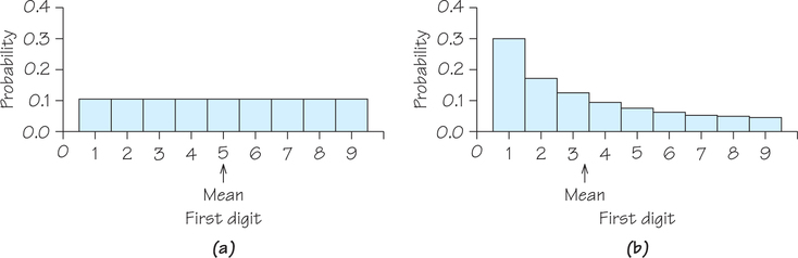
The comparison of means between Benford’s law and random digits, $3.441 < 5$ , reflects the greater probability of smaller first digits under Benford’s law. Probability histograms for these two models appear in Figure 8.21. Because the histogram for random digits (Figure 8.21a) is symmetric, the mean lies at the center of symmetry. We can’t determine the mean of the right-skewed Benford’s law model precisely by simply looking at Figure 8.21b; calculation is needed.

Figure 8.21 Probability histograms of two models for first digits in numerical records. The mean of each distribution is marked. (a) Digits are equally likely, (b) Digits follow Benford’s law.

Self Check 14

A small business finds that the number of employees who call in sick on any given day can be described by the following probability model. Calculate the mean number of employees who call in sick on any given day.

Number who call in sick, $x$	0	1	2	3	4
Probability, $p$	0.49	0.26	0.15	0.07	0.03

Using products from the table below:

$μ - 0 + 0.26 + 0.30 + 0.21 + 0.12 = 0.89$

Number who call in sick, $x$	0	1	2	3	4
Probability, $p$	0.49	0.26	0.15	0.07	0.03
Product, $x \cdot p$	0	0.26	0.30	0.21	0.12

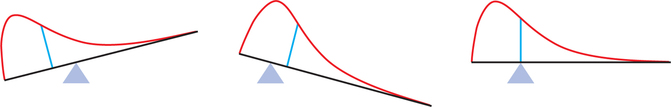
What about continuous probability models? Think of the area under a density curve as being cut out of solid homogenous material. The mean $μ$ is the point at which the shape would balance. Figure 8.22 illustrates this interpretation of the mean. The mean lies at the center of symmetric density curves, such as the uniform density in Figure 8.18 (page 372) and the normal curve in Figure 8.20 (page 374). Exact calculation of the mean of a distribution with a skewed density curve requires advanced mathematics.

Page 378

Figure 8.22 The mean of a continuous probability model is the “balance point” for the density curve.

The mean $μ$ is an average outcome in two senses. The definition for discrete probability models says that it is the average of the possible outcomes weighted by their probabilities. More likely outcomes get more weight in the average. An important fact of probability, the law of large numbers, says that $μ$ is the average outcome in another sense as well.

Law of Large Numbers THEOREM

Observe any random phenomenon having numerical outcomes with finite mean $μ$ . According to the law of large numbers, as the phenomenon is repeated a large number of times, the following occurs:

The proportion of trials in which an outcome occurs gets closer and closer to the probability of that outcome.
The mean $\bar{x}$ of the observed values gets closer and closer to $μ$ .

EXAMPLE 22 The Law of Large Numbers and the Gambling Business

The law of large numbers explains why gambling can be a business. In a casino, the house (i.e., the casino) always has the upper hand. Even when the edge is very small, such as in blackjack—where according to “The Wizard of Odds,” the house edge is only around 0.3%—the casino makes money. The house edge is defined as the ratio of the average loss to the initial bet. That means for every $10 initial bet, the gambler will lose, on average, $0.003 \times $ 10 = $ 0.03$ , or 3 cents per game. Over thousands and thousands of gamblers and games, that small edge starts to generate big revenues. Unlike most gamblers, casinos are playing the long game and not just hoping for a short-term payout.

The winnings (or losses) of a gambler on a few plays are highly variable or uncertain; that’s why gambling is exciting. It is only in the long run that the mean outcome is predictable. Take, for example, roulette. An American roulette wheel has 38 slots, with numbers 1 through 36 (not in order) on alternating red and black slots and 0 and 0 on two green slots. The dealer spins the wheel and whirls a small ball in the opposite direction within the wheel. Gamblers bet on where the ball will come to rest (see Figure 8.23). One of the simplest wagers is to choose red. A bet of $1 on red pays off an additional $1 if the ball lands in a red slot. Otherwise, the player loses the $1.

Figure 8.23 One round of blackjack and roulette. (a) A winning hand in blackjack! (b) Red wins!

Page 379

Lou bets on red. He wins if the ball stops in one of the 18 red slots. He loses if it lands in one of the 20 slots that are black or green. Because casino roulette wheels are carefully balanced so that all slots are equally likely, the probability model is

Net Outcome for Gambler

$\begin{array}{l} Win $ 1 & Lose $ 1 \\ Probability \frac{18}{33} = 0.474 & \frac{20}{38} = 0.526 \end{array}$

The mean outcome of a single $1 bet on red is

$\begin{array}{l} μ = ($ 1) (\frac{18}{38}) + (- $ 1) (\frac{20}{38}) \\ = - $ \frac{2}{38} = - $ 0.053 (a loss of 5.3 cents) \end{array}$

The law of large numbers says that the mean $μ$ is the average outcome of a very large number of individual bets. In the long run, gamblers will lose (and the casino will win) an average of 5.3 cents per bet.

So the house, unlike individual gamblers, can count on the long-run regularity described by the law of large numbers. The average winnings of the house on tens of thousands of plays will be very close to the mean of the distribution of winnings. Needless to say, gambling games have mean outcomes that guarantee the house a profit; though, as we have seen, some games such as blackjack give the house a smaller advantage than others such as keno. (According to “The Wizard of Odds,” the house edge on keno is 25% to 29%!)

Self Check 15

On the roulette wheel described in Example 22, you can also bet on the ball landing on the numbers 1 through 12, in which case the payout is $2 on an initial bet of $1.

What is the probability that the gambler wins? Loses?
- $P (win) = 12 / 38 \approx 0.3158$ ; the gambler wins 31.58% of the time over many, many games. $P (loss) = 1 - P (win) \approx 0.6842$ ; the gambler loses 68.42% of the time over many, many games.
For each $1 bet, what are the expected winnings for the house (or losses for the gambler)? How does the house edge in this game compare with the house edge in betting on red?
- $(- 1) (0.6842) + (2) (0.3158) = - 0.0526$ ; the house edge is exactly the same as for betting on red.

We know that the simplest description of a distribution of data requires both a measure of center and a measure of variability. The same is true for probability models. The mean is the average value for both a set of data and a discrete probability model. All the observations are weighted equally in finding the mean $\bar{x}$ for data, but the values are weighted by their probabilities in finding the mean $μ$ of a probability model. The measure of variability that goes with the mean is the standard deviation. In Section 5.7, on page 203, we learned that the standard deviation $s$ of data is the square root of the average squared deviation of the observations from their mean. We apply exactly the same idea to probability models, using probabilities as weights in the average. Here is the definition.

Standard Deviation of a Discrete Probability Model DEFINITION

Suppose that the possible outcomes $x_{1}, x_{2}, \dots, x_{k}$ in a sample space $S$ are numbers, and that $p_{j}$ is the probability of outcome $x_{j}$ . The standard deviation of a discrete probability model with mean $μ$ is denoted by the lowercase Greek letter sigma ( $σ$ ) and is given by this formula:

$σ = \sqrt{{(x_{1} - μ)}^{2} p_{1} + {(x_{2} - μ)}^{2} p_{2} + \dots + {(x_{k} - μ)}^{2} p_{k}}$

Page 380

EXAMPLE 23 Standard Deviation of the Probability Model for benford’s Law

If the first digits in a set of records obey Benford’s law, the discrete probability model is as follows:

First digit	1	2	3	4	5	6	7	8	9
Probability	0.301	0.176	0.125	0.097	0.079	0.067	0.058	0.051	0.046

We saw in Example 21 that the mean is $μ = 3.441$ . To find the standard deviation,

$\begin{matrix} σ = \sqrt{{(x_{1} - μ)}^{2} ρ_{1} + {(x_{2} - μ)}^{2} ρ_{2} + \dots + {(x_{k} - μ)}^{2} ρ_{k}} \\ = \sqrt{{(1 - 3.441)}^{2} (0.301) + {(2 - 3.441)}^{2} (0.176) + \dots + {(9 - 3.441)}^{2} (0.046)} \\ = \sqrt{1.7935 + 0.3655 + \dots + 1.4215} \\ = \sqrt{6.061 \approx 2.46} \end{matrix}$

You can follow the same pattern to find the standard deviation of the equally likely model and show that the Benford’s law model, by virtue of clustering near the left side, has less variability than the equally likely model.

Self Check 16

Return to the distribution of net outcomes for betting on red at the roulette wheel from Example 22 (page 378). You know that $μ = - 0.053$ . Find the standard deviation for a single $1 bet on red.

$\begin{matrix} σ = \sqrt{{(1 - (- 0.053))}^{2} \frac{18}{38} + {(- 1 - (0.053))}^{2} \frac{20}{38}} \\ = \sqrt{{(1.053)}^{2} \frac{18}{38} + {(- 0947)}^{2} \frac{20}{38}} \\ = \sqrt{0.9972} \approx $ 0.9986 \end{matrix}$

Finding the standard deviation of a continuous probability model usually requires advanced mathematics (calculus). Section 5.8 provided the answer in one important case (see page 213): The standard deviation of a normal curve is the distance from the center (the mean) to the change-of-curvature point on either side.