10.2 Direct Price Discrimination I: Perfect/First-Degree Price Discrimination
When to Use It Perfect/First-Degree Price Discrimination
The firm has market power and can prevent resale.
The firm’s customers have different demand curves.
The firm has complete information about every customer and can identify each one’s demand before purchase.
direct price discrimination
A pricing strategy in which firms charge different prices to different customers based on observable characteristics of the customers.
Let’s start our study of pricing strategies by looking at a firm that has market power, can prevent resale, and knows that its consumers differ in their willingness to pay and therefore have different demand curves. To choose a price-
perfect price discrimination (first-
A type of direct price discrimination in which a firm charges each customer exactly his willingness to pay.
Let’s first consider the possibilities for a firm that has so much information about its customers before they buy that it knows each individual buyer’s demand curve and can charge each buyer a different price equal to the buyer’s willingness to pay. This type of direct price discrimination is known as perfect price discrimination or first-
Suppose a firm faces a market demand curve like the one labeled D in Figure 10.2. Panel a shows the outcomes for a perfectly competitive firm and a monopolistic firm. We know from Chapter 8 that in a perfectly competitive market, the equilibrium price (which is the same as MR in that case) equals marginal cost MC and the firm produces quantity Qc. Consumer surplus is the area under the demand curve and above the price, A + B + C. Because we assume that marginal cost is constant, there is no producer surplus.
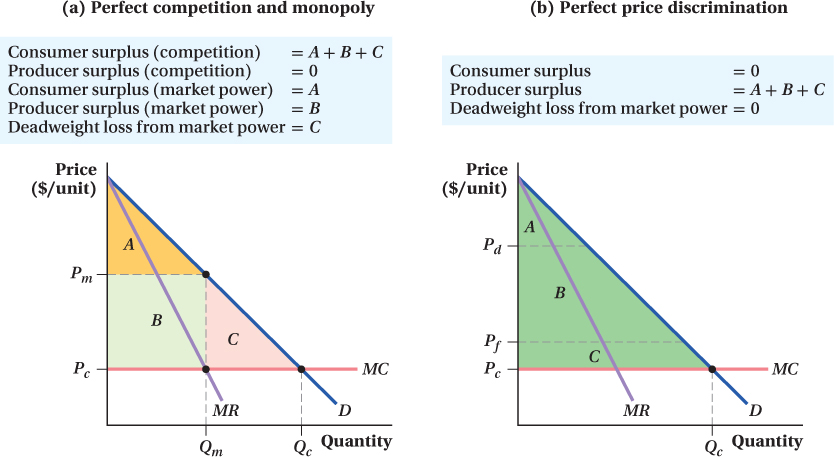
(b) If a firm with market power can identify each customer’s demand curve, then it will charge each customer her willingness to pay and capture the entire surplus, A + B + C. For example, the firm will charge a customer willing to pay Pd exactly the price Pd and a customer willing to pay Pf the price Pf. The firm will sell up to the quantity Qc, the perfectly competitive quantity where Pc = MC. There is no deadweight loss when a firm practices perfect price discrimination.
381
In Chapter 9, we saw that a firm with market power facing demand curve D and with no ability to prevent resale produces the quantity where its marginal cost equals its marginal revenue, Qm, and sets the price Pm for that quantity from its demand curve. It charges this single price to everyone in the market. This market power pricing has three outcomes relative to the competitive pricing: (1) There is now a producer surplus equal to the rectangle B (far better from the firm’s perspective than the competitive outcome, no producer surplus); (2) there is now a deadweight loss equal to the triangle C, because quantity is below its competitive level; and (3) consumer surplus is reduced to area A.
If, however, the firm with market power can prevent resale and directly identify each and every customer’s demand curve (panel b), the outcome is very different. In this case, the firm can charge every customer her willingness to pay for every unit (or, to guarantee she’d take the deal, just a bit below this level). This is perfect price discrimination, and the benefit to the firm is tremendous. For any unit of output where a customer’s willingness to pay is greater than the firm’s marginal cost of producing it, the firm captures the whole amount of available surplus. So, for example, a customer accounting for the portion of the demand curve at Pd pays that relatively high price, while another at Pf pays that relatively low price. In these and all other cases, even though the prices are different, customers pay the most they are willing to pay, and the firm gets the entire surplus (the area below demand and above marginal cost).
382
After all such transactions, the firm will have sold a quantity of Qc to various consumers at different prices depending on each buyer’s willingness to pay. (Because the firm can prevent resale, customers aren’t able to buy the product from another customer for a lower price than the firm offers.) The producer surplus the firm earns as a result equals the entire surplus in the market, A + B + C. This is the maximum amount of surplus that can be made from the market because no consumer will pay more than her willingness to pay (which rules out the area above the demand curve) and the firm must pay its costs (which eliminates the area below the marginal cost curve). A firm that can perfectly price-
Another interesting feature of perfect price discrimination is that, unlike the single-
figure it out 10.1
A firm with market power faces an inverse demand curve for its product of P = 100 – 10Q. Assume that the firm faces a marginal cost curve of MC = 10 + 10Q.
If the firm cannot price-
discriminate, what is the profit- maximizing level of output and price? If the firm cannot price-
discriminate, what are the levels of consumer and producer surplus in the market, assuming the firm maximizes its profit? Calculate the deadweight loss from market power. If the firm has the ability to practice perfect price discrimination, what is the firm’s output?
If the firm practices perfect price discrimination, what are the levels of consumer and producer surplus? What is the deadweight loss from market power?
Solution:
If the firm cannot price-
discriminate, it maximizes profit by producing where MR = MC. If the inverse demand function is P = 100 – 10Q, then the marginal revenue must be MR = 100 – 20Q. (Remember that, for any linear inverse demand function P = a – bQ, marginal revenue is MR = a – 2bQ.) Setting MR = MC, we obtain
100 – 20Q = 10 + 10Q
90 = 30Q
Q* = 3
To find the optimal price, we plug Q = 3 into the inverse demand equation:
P* = 100 – 10Q*
= 100 – 10(3)
= 100 – 30
= 70
The firm sells 3 units at a price of $70 each.
To find consumer and producer surplus, we need to start with a diagram showing the demand, marginal revenue, and marginal cost curves:
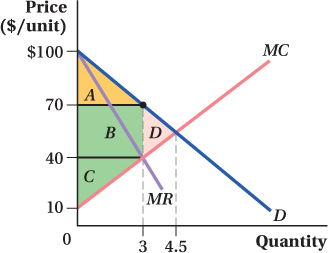
Consumer surplus is the area above price and below demand (area A). Producer surplus is the area above marginal cost but below the price (area B + C). (Note that we could just label these two areas as a large trapezoid, but it is easier to remember the formulas for the area of a rectangle and a triangle!) We can calculate the areas:
383
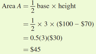
Consumer surplus is $45.
Area B = base × height
To get the height of areas B and C, we need the MC of producing a quantity of 3: MC = 10 + 10Q = 10 + 10(3) = $40. So,
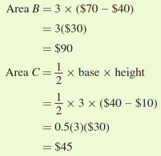
Thus, Producer surplus = area B + area C = $90 + $45 = $135.
The deadweight loss from market power is the loss in surplus that occurs because the market is not producing the competitive quantity. To calculate the competitive quantity, we set P = MC:
100 – 10Q = 10 + 10Q
90 = 20Q
Q = 4.5
The deadweight loss can be seen on the diagram as area D:
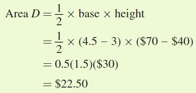
The deadweight loss from market power is $22.50.
If the firm practices perfect price discrimination, it will produce where P = MC. As we saw in part (b) above, this means that the firm will produce 4.5 units.
If the firm practices perfect price discrimination, consumer surplus will be zero because every consumer will be charged a price equal to his willingness to pay. Producer surplus will be the full area between the demand curve and the marginal cost curve (area A + B + C + D):
Producer surplus = area A + area B + area C + area D
= $45 + $90 + $45 + $22.50
= $202.50
There is no deadweight loss when the firm perfectly price-
discriminates. The competitive output level is achieved (Q = 4.5). Producers end up with the entire surplus available in the market.
Examples of Perfect Price Discrimination
Actual cases of died-
When people walk into a car dealership, the salesperson sizes them up and eventually begins negotiating over price. While the dealer doesn’t have complete information about each customer’s willingness to pay, haggling differently with every customer is a lot like perfect price discrimination—
Likewise, families applying for college financial aid are required to submit complete information about their assets and income along with the student’s assets and income. From this information, the school has an almost perfect understanding of each student’s willingness to pay. This allows schools to produce an individually tailored financial aid plan. But that is another way of saying that they charge a different tuition price to each student, depending on how much they think the student can afford.
384
Application: How Priceline Learned That You Can’t Price-Discriminate without Market Power
Priceline is the online travel service known, in part, for originating the “name your own price” model of online sales. The initial idea was that people would go to Priceline’s site and enter what they were willing to pay for an airplane ticket—
The idea was that by asking each person what she was willing to pay, Priceline could engage in something like perfect price discrimination and therefore make a lot of money. We can think of its original business model in terms of Figure 10.3. Priceline figured that, with a marginal cost of tickets of MC and travelers’ willingness to pay (demand curve) at D, it stood to earn producer surplus approximately equal to the area A + B. The stock market liked this model, too: Within three years of starting up its Web site, the company was valued at $13 billion, more than several of the major airlines combined.
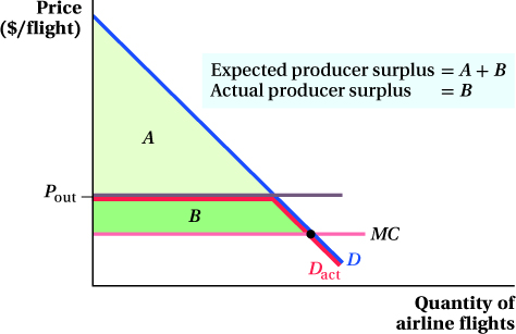
There was a serious problem in Priceline’s approach, however. Priceline wanted to price-
Priceline’s problem was that, because travelers could also get fares at low prices directly from other travel sites, they wouldn’t offer their true willingness to pay from their demand curves. Instead, customers would only offer to buy tickets at a lower price than they could buy them elsewhere.
385
Priceline’s market demand curve was therefore not the consumer’s demand curve D, but rather a curve strictly below the market price of tickets at other sites. In the figure, the outside price occurs at Pout. So, the actual demand curve facing Priceline was not D but Dact instead. This kind of price discrimination doesn’t make large profits. It left Priceline with a surplus of only B, the small area below the actual demand curve and above marginal cost. Indeed, this demand curve left Priceline with less producer surplus than that earned by other travel sites (which were charging prices at or above Pout).
Realizing this, Priceline eventually deemphasized the “name your own price” business model and expanded into the conventionally priced online travel business. It has so far succeeded—
 See the problem worked out using calculus