13.2 Supply in a Perfectly Competitive Factor Market
In a perfectly competitive market, labor supply at the firm level is straightforward. Because the firm can hire as much labor as it wants at the market wage, it faces a perfectly elastic supply of labor at the market wage. All shifts in the firm’s labor demand will show up as changes in the quantity of labor hired rather than changes in the wage. The supply of labor available to firms in the labor market depends on the collective willingness of people to work. A person’s willingness to work depends on his age, family situation, health, and many other factors. As with any supply curve, we hold all these other things constant and focus on the effect of the wage on the quantity of labor supplied. To understand what market-level labor supply looks like, then, we have to understand how people’s willingness to work changes when the wage changes.
Work, Leisure, and Individual Labor Supply
A key to grasping how wages affect people’s labor supply is to understand how they think about leisure time. For just about everyone, leisure is a good, just like cell phones or massages. Consuming more of it raises people’s utility.
If leisure is a good, what is its price? Consuming leisure involves using up time. The price of leisure is what a person (call her Marissa) could be doing with that time if she wasn’t being leisurely—that is, working. (Economists often consider any time a person spends not working as leisure, whether or not he or she is doing something we might think of as leisurely. One of our colleagues likes to jokingly, but truthfully, remind students that the time they spend attending lectures is considered leisure because they aren’t earning wages for doing so.)
The benefit of working, aside from any inherent pleasure Marissa might get from her job, is the income she earns from it—or more precisely, the utility she obtains by consuming goods and services bought with her work income. By choosing to enjoy more leisure, Marissa gives up the income she could have earned had she worked during that leisure time. That lost income equals her wage rate. So the wage, and the goods and services that she could have bought with her income, are her price of leisure.
We can think of Marissa’s labor supply as involving a choice between consuming leisure and consuming the goods and services that can be bought with her income from work. If we treat those other goods and services as a single good (let’s call it “consumption” for short, with its quantity measured in dollars), the relative price between leisure and consumption is the wage. If Marissa’s wage is $30 per hour, for example, and she chooses to take one more hour of leisure (i.e., work one hour less), she gives up $30 in consumption.
We can describe the work–leisure choice using the set of tools we utilized in Chapter 4: Marissa has a utility function that depends on both the amount of leisure time she spends and the consumption she enjoys from her work income. She maximizes her utility subject to a budget constraint for which the relative price of leisure and consumption is her wage rate. This is illustrated in Figure 13.5, which looks at Marissa’s choice of how many hours to work in a day. (We could easily look at consumption–leisure choices over different periods than a day—say, a week or a year—if we wanted to; the analysis would be qualitatively the same).
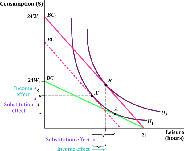
Figure 13.5: FIGURE 13.5 The Consumption–Leisure Choice
Figure 13.5: An increase in the wage from W1 to W2 shifts the budget constraint from BC1 to BC2, and the optimal consumption–leisure bundle changes from A to B. The substitution effect of the wage increase, which decreases leisure and increases consumption because leisure has become relatively more costly, accounts for the shift from bundle A to A′, the tangency of U1 and BC′. The shift from A′ to B is the income effect.
The most leisure Marissa could take in a day is 24 hours. If she does, she won’t earn any wages that day, and her consumption will be $0. Therefore, we know the budget constraint must include the point for 24 hours of leisure and $0 of consumption. This is the budget constraint’s horizontal intercept. If she instead chooses to take no leisure and work the entire 24-hour period, she will maximize her consumption at 24 × W1, where W1 is her wage. Thus, another point on the budget constraint BC1 is 0 hours of leisure and $24W1 of consumption, the vertical intercept of the constraint. Because Marissa must give up $W1 of consumption for each hour of leisure she takes, the budget constraint’s slope is –W1.
An indifference curve U1 from Marissa’s utility function for consumption and leisure is shown in the figure. Marissa’s optimal consumption and leisure bundle is at the tangency of U1 and the budget constraint BC1, point A.
Suppose the wage rises to W2. This rotates the budget constraint around the horizontal intercept (a different wage doesn’t change the fact that Marissa can take at most 24 hours of leisure in a day), as shown in Figure 13.5. At any other leisure choice, however, Marissa can now have a higher level of consumption. The increase in wage shifts Marissa’s optimal consumption–leisure bundle to the tangency of indifference curve U2 and the new budget line BC2, point B.
Income and Substitution Effects of a Change in Wages
A higher wage has two effects on Marissa’s consumption and leisure choices. First, leisure now has a higher price relative to consumption; working one less hour has become more expensive for Marissa in terms of forgone consumption. This substitution effect pushes her to choose less leisure (i.e., work more) and consume more goods and services. (If her wage were to fall instead, it would make leisure relatively cheaper and she would choose to work fewer hours.)
But there is another effect of an increase in the wage that we hinted at before. For any given level of work—or equivalently, any given level of leisure time—it raises Marissa’s income. This means there is also an income effect of a wage increase, not just a substitution effect. For Marissa as with most people, leisure is a normal good, so she will consume more of it as her income rises—the opposite of the substitution effect.
These two effects are the same ones we saw for price changes in Chapter 4. As we did there, we can decompose the total change in consumption and leisure into the separate influences of the substitution and income effects. To do so, remember that we need to figure out what Marissa’s optimal consumption–leisure bundle would be if the relative prices had changed but her income hadn’t (i.e., if the substitution effect of the wage change applied but the income effect didn’t). We can do this by finding a budget constraint that is parallel to the new post-wage-increase budget constraint but is tangent to the original indifference curve U1. This is the dashed line BC′ in Figure 13.5. The tangency point A′ shows the bundle Marissa would choose at the new relative price but without the income effect; in other words, it isolates the influence of substitution effect. The difference in the bundles A and A′ reflects the substitution effect of the wage increase on Marissa’s consumption and leisure choices. The difference between A′ and B reflects the income effect of the higher wage.
The substitution effect makes Marissa’s labor supply curve, which shows how much she is willing to work at any given wage level, slope up. This shape is how we usually think of supply curves for anything: The higher the price of the good (here, the wage), the higher the quantity of the product (work hours) the producer (Marissa) will supply.
Backward-Bending Supply Curves
The net effect of a wage change on how much she is willing to work is the difference between the income and substitution effects. In principle, at least, if the income effect is large enough, there would be a negative relationship between wages and how much Marissa is willing to work, and her labor supply curve would no longer slope up. An example of this outcome is shown in Figure 13.6. At wages below WBB, the substitution effect dominates; increases in the wage will make Marissa willing to work more. Above WBB, however, the income effect begins to dominate, and the quantity of work she is willing to supply falls as wages rise. Economists call labor supply curves with this negative slope backward-bending labor supply curves.
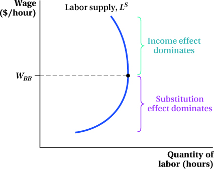
Figure 13.6: FIGURE 13.6 Backward-Bending Labor Supply
Figure 13.6: At wages below WBB, the substitution effect dominates: Individuals work more (and consume less leisure) as the wage increases, and the quantity of labor supplied rises. Above WBB, the income effect begins to dominate: Individuals work less (and consume more leisure) as the wage increases, and the quantity of labor supplied falls.
Economists have found examples of backward-bending labor supply curves in certain markets. In one broad-ranging case, economic historian Dora Costa gathered surveys on the work habits of thousands of U.S. men working in the 1890s.1 She found that low-wage workers spent more hours per day working than those earning high wages. Specifically, workers in the lowest wage decile (those being paid wages in the lowest 10% of all observed wage rates) averaged 11.1 hours of work per day, but those in the top wage decile (the top 10% of wage rates) only worked 8.9 hours per day. Workers in the highest wage group worked 5% fewer hours than those being paid the median wage, who in turn worked 14% less than those in the lowest wage group. In other words, the daily labor supply curve appeared to exhibit backward-bending patterns. (Interestingly, using other data, Costa also showed that the pattern had reversed itself by the 1990s. While workers in that period across the wage scale spent, on average, less time per day working than a century before, now those at the high end of the scale worked more than those at the low end.)
The net effect of wage changes on labor supply is the sum of the substitution and income effects. As explained in the Application below, economists have found evidence of backward-bending labor supply behavior among certain workers at certain times.
Application: Tiger Woods’s Backward-Bending Labor Supply Curve
Tiger Woods is perhaps the most recognizable face in professional golf. He’s won 79 PGA tour events and picked up 14 Majors. He’s lent his name to product endorsement campaigns for which he’s taken home tens of millions of dollars. But it’s not just his athletic skill that separates him from the average American laborer: He’s probably one of the rare set of workers facing week-to-week wages on the backward-bending portion of his labor supply curve. In other words, as his wages increase, he actually decreases the number of tournaments in which he plays.

Tiger Woods supplying labor.
Andrew Redington/Getty Images
PGA rules allow each golfer to elect which and how many events to play in, meaning the athlete considers the labor–leisure tradeoff separately for each tournament event. With tournament payoffs in the millions of dollars for just four rounds of golf, who wouldn’t play? Indeed, most golfers do. Generally, around 100 players sign up for any given event. This doesn’t even include the over 1,000 hopefuls who play in brutal qualifying rounds, vying for just 25 spots on the PGA Tour.
Given the opportunity, these hopefuls would gladly play every tournament, but as economists Otis Gilley and Marc Chopin discovered, players like Tiger Woods don’t.2 Gilley and Chopin looked at how low- and middle-income PGA players in the 1990s responded to increases in their wages and compared this result to the effects of wage increases on high-income players. Whereas low-level players entered more events as their event winnings increased, golfers at the top of their game decreased their tournament play as their wages increased. Top golfers were operating on the backward-bending portion of their labor supply curves. In particular, for every $1,000 increase in expected per-event winnings, the number of tournaments entered in a season by high-income players decreased by 0.05 to 0.1. For these select players, the income effect dominated the substitution effect, and, faced with the leisure–labor tradeoff, they elected to consume more leisure.
Workers in other fields—including some economists—often spend their leisure time on the golf course. But for a professional golfer, a day on the green is work, not leisure. So just what does a PGA player do on his day off? Gilley and Chopin found that married golfers took more days off than did single golfers. Drawing on their own experiences as family men, the two hard-working economists concluded that golfers must be taking off work to spend more quality time with their wives and kids. The example of Tiger Woods, however, shows that not all predictions of economic theory hold up in the real world. 
Market-Level Labor Supply
The market-level labor supply curve shows the total amount of labor all workers are willing to supply at every possible wage. In other words, it is the horizontal sum of every worker’s labor supply curve. To construct it, we fix a wage, figure out each worker’s quantity of labor supplied at that wage, and add up those quantities. Once we’ve done this for every possible wage, we have found the market-level labor supply curve.
We discussed earlier how it is possible that individual workers’ labor supply curves can be backward-bending. In principle, the market-level labor supply curve can be backward-bending, too. However, most available evidence suggests that at the market level, the substitution effect dominates so there is no backward bend. Backward-bending labor supply is unlikely at the market level because, even if an individual like Marissa hits the point where her quantity of labor supply will fall if her wage rises higher, there are usually many other people willing to supply more labor at those high wages (whether that’s because they add more hours to the number they’re already working or, if they weren’t working before, decide to start working) to counteract the income effects of Marissa and those like her who cut back on their work hours. Thus, although an individual’s labor supply may sometimes bend backward, the market labor supply curve usually slopes up because the total quantity of labor supplied by all workers increases as the wage rises.