2.5 Elasticity
Mathematically, the slopes of demand and supply curves relate changes in price to changes in quantity demanded or quantity supplied. Steeper curves mean that price changes are correlated with relatively small quantity changes. When demand curves are steep, this implies that consumers are not very price-
39
elasticity
The ratio of the percentage change in one value to the percentage change in another.
price elasticity of demand
The percentage change in quantity demanded resulting from a given percentage change in price.
The concept of elasticity expresses the responsiveness of one value to changes in another (and here specifically, the responsiveness of quantities to prices). An elasticity relates the percentage change in one value to the percentage change in another. So, for example, when we talk about the sensitivity of consumers’ quantity demanded to price, we refer to the price elasticity of demand: the percentage change in quantity demanded resulting from a given percentage change in price.
Slope and Elasticity Are Not the Same
You might be thinking that the price elasticity of demand sounds a lot like the slope of the demand curve: how much quantity demanded changes when price does. While elasticity and slope are certainly related, they’re not the same.
The slope relates a change in one level (prices) to another level (quantity). The demand curve we introduced in the tomato example was Q = 1,000 – 200P. The slope of this demand curve is –200; that is, quantity demanded falls by 200 pounds for every dollar per pound increase in price.
There are two big problems with using just the slopes of demand and supply curves to measure price responsiveness. First, slopes depend on the units of measurement. If we measured tomato prices P in cents per pound rather than dollars, the demand curve would be Q = 1,000 – 2P, because the quantity of tomatoes demanded would fall by 2 pounds for every 1 cent increase in price. But the fact that the coefficient on P is now 2 instead of 200 doesn’t mean that consumers are 1/100th as price-
Using elasticities to express responsiveness avoids these tricky issues, because everything is expressed in relative percentage changes. That eliminates the units problem (a 10% change is a 10% change regardless of what units the thing changing is measured in) and makes magnitudes comparable across markets.
The Price Elasticities of Demand and Supply
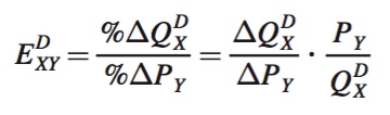
The price elasticity of demand is the ratio of the percentage change in quantity demanded to an associated percentage change in price. Mathematically, its formula is
Price elasticity of demand = (% change in quantity demanded)/(% change in price)
The price elasticity of supply is exactly analogous:
Price elasticity of supply = (% change in quantity supplied)/(% change in price)
40
To keep the equations simpler from now on, we’ll use some shorthand notation. ED will denote the price elasticity of demand, ES the price elasticity of supply, %ΔQD and %ΔQS the percentage change in quantities demanded and supplied, respectively, and %ΔP the percentage change in price. In this shorthand, the two equations above become
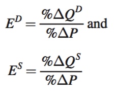
So, for example, if the quantity demanded of a good falls by 10% in response to a 4% price increase, the good’s price elasticity of demand is ED = –10%/4% = –2.5. There are a couple of things to note about this example. First, because demand curves slope downward, the price elasticity of demand is always negative (or more precisely, always nonpositive; in special cases that we discuss later, it can be zero). Second, because it is a ratio, a price elasticity can also be thought of as the percentage change in quantity demanded for a 1% increase in price. That is, for this good, a 1% increase in price leads to a –2.5% change in quantity demanded.
The price elasticity of supply works exactly the same way. If producers’ quantity supplied increases by 25% in response to a 50% increase in price, for example, the price elasticity of supply is ES = 25%/50% = 0.5. The price elasticity of supply is always positive (or again more precisely, always nonnegative) because quantity supplied increases when a good’s price rises. And just as with demand elasticities, supply elasticities can be thought of as the percentage change in quantity in response to a 1% increase in price.
Price Elasticities and Price Responsiveness
Now that we’ve defined elasticities, let’s use them to think about how responsive quantities demanded and supplied are to price changes.
When demand (supply) is very price-
Examples of markets with large-
Markets with less price-
Markets with large price elasticities of supply—
41
Markets with low price elasticities of supply have quantities supplied that are fairly unresponsive to price changes. This would occur in markets where it is costly for producers to vary their production levels, or it is difficult for producers to enter or exit the market. The supply curve for tickets to the Super Bowl might have a very low price elasticity of supply because there are only so many seats in the stadium. If the ticket price rises today, the stadium owners can’t really put in additional seats. The supply elasticity in this market might be close to zero. It’s probably slightly positive, however, because the owners could open some obstructed-
Application: Demand Elasticities and the Availability of Substitutes
We discussed how the availability of substitutes can affect the price elasticity of demand. When consumers can easily switch to other products or markets, they will be more responsive to changes in the price of a particular good. This means that, for any small rise in price, there will be a large decline in quantity demanded and the price elasticity of demand will be relatively large (in absolute value).
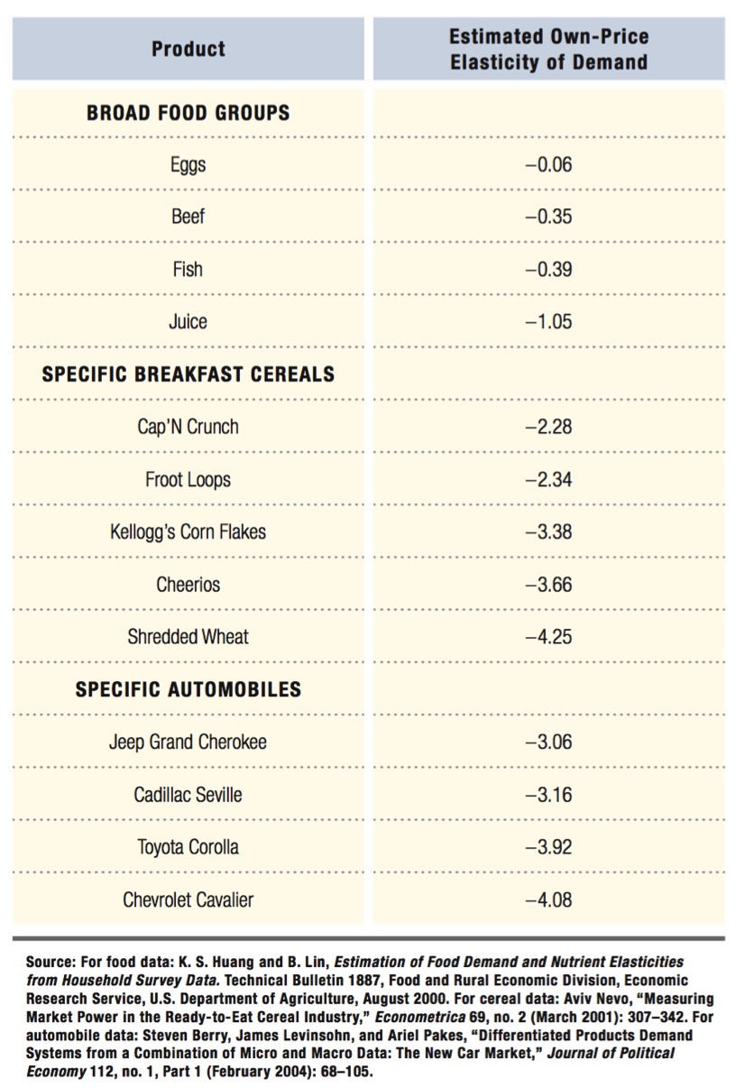
Table 2.3 presents some other elasticities estimated by economists for various goods. Larger groupings like “juice” or “beef” tend to have inelastic demand. The more narrowly defined the goods are (and so the more substitute products there are), the more elastic the demand tends to be. Thus, the elasticity of beef is only –0.35, whereas the elasticity of Shredded Wheat brand breakfast cereal is –4.25.
Economists Glenn and Sara Ellison found an extreme example of the effect of substitution possibilities and extreme demand elasticities to match.8 They looked at the markets for different CPUs and memory chips on a price search engine Web site. The Web site collects price quotes for specific computer chips and chipsets from hardware suppliers and then groups the quotes together (ranked by price) with links to the corresponding suppliers. The search engine makes it extremely easy to compare multiple suppliers’ prices for identical products. Because the product in this case is so standardized, little distinguishes one chip from another. As a result, consumers are able and willing to respond strongly to any price differences across the suppliers of the chips.
This easy ability for consumers to substitute across suppliers means the demand curve for any given supplier’s CPUs and memory chips is extremely elastic. If a supplier’s price is even slightly higher than that of its competitors, consumers can easily buy from someone else. Ellison and Ellison, using data collected from the Web site, estimated the price elasticity of demand for any single chip to be on the order of –25. In other words, if the supplier raises its price just 1% higher than that of its competitors (which works out to a dollar or two for the chips listed on the Web site), it can expect sales to fall by 25%! This huge price response is due to the many substitution possibilities the search engine makes available to consumers. Thus, the availability of substitutes is one of the key determinants of the price elasticity of demand. 
42
Elasticities and Time Horizons Often, a key factor determining the flexibility consumers and producers have to respond to price differences, and therefore the price elasticity of their quantities demanded and supplied, is the time horizon.
43
In the short run, consumers are often limited in their ability to change their consumption patterns, but given more time, they can make adjustments that give them greater flexibility. The classic example of this is in the market for gasoline. If there is a sudden price spike, many consumers are essentially stuck having to consume roughly the same quantity of gas as they did before the price spike. After all, they have the same car, the same commute, and the same schedule as before. Maybe they can double up on a few trips, or carpool more often, but their ability to respond to prices is limited. For this reason, the short-
The same logic holds for producers and supply elasticities. The longer the horizon, the more options they have to adjust output to price changes. Manufacturers already producing at capacity might not be able to increase their output much in the short run if prices increase, even though they would like to. If prices stay high, however, they can hire more workers, build larger factories, and new firms can set up their own production operations and enter the market.
For these reasons, the price elasticities of demand and supply for most products are larger in magnitude (i.e., more negative for demand and more positive for supply) in the long run than in the short run. As we see in the next section, larger-
elastic
A price elasticity with an absolute value greater than 1.
inelastic
A price elasticity with an absolute value less than 1.
unit elastic
A price elasticity with an absolute value equal to 1.
perfectly inelastic
A price elasticity that is equal to zero; there is no change in quantity demanded or supplied for any change in price.
perfectly elastic
A price elasticity that is infinite; any change in price leads to an infinite change in quantity demanded or supplied.
Classifying Elasticities by Magnitude Economists have special terms for elasticities of particular magnitudes. Elasticities with magnitudes (in absolute value) greater than 1 are referred to as elastic. In the above examples, apples have elastic demand and software has elastic supply. Elasticities with magnitudes less than 1 are referred to as inelastic. The demand for circus candy and the supply of Super Bowl tickets are inelastic. If the price elasticity of demand is exactly –1, or the price elasticity of supply is exactly 1, this is referred to as unit elastic. If price elasticities are zero—
Elasticities and Linear Demand and Supply Curves
As we discussed above, economists often use linear (straight-
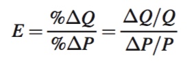
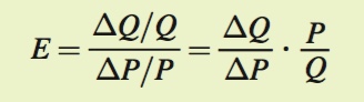
We can rewrite the elasticity formula in a way that makes it easier to see the relationship between elasticity and the slope of a demand or supply curve. A percentage change in quantity (%ΔQ) is the change in quantity (ΔQ) divided by the original quantity level Q. That is, %ΔQ = ΔQ/Q. Similarly, the percentage change in price is %ΔP = ΔP/P. Substituting these into the elasticity expression from above, we have
44
where E is a demand or supply elasticity, depending on whether Q denotes quantity demanded or supplied.
Rearranging terms yields
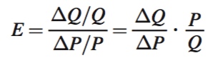
or
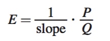
where “slope” refers to ΔP/ΔQ, the slope of the demand or supply curve in the standard price-
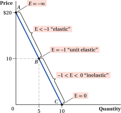
Elasticity of a Linear Demand Curve Suppose we’re dealing with the demand curve in Figure 2.15. Its slope is –2, but its elasticity varies as we move along it because P/Q does. Think first about the point A, where it intercepts the vertical axis. At Q = 0, P/Q is infinite because P is positive ($20) and Q is zero. This, combined with the fact that the curve’s (constant) slope is negative, means the price elasticity of demand is –∞ at this point. The logic behind this is that consumers don’t demand any units of the good at A when its price is $20, but if price falls at all, their quantity demanded will become positive, if still small. Even though this change in quantity demanded is small in numbers of units of the good, the percentage change in consumption is infinite, because it’s rising from zero.
45
As we move down along the demand curve, the P/Q ratio falls, reducing the magnitude of the price elasticity of demand. (Remember, the slope isn’t changing, so that part of the elasticity stays the same.) It will remain elastic—
To recap, the price elasticity of demand changes from –∞ to zero as we move down and to the right along a linear demand curve.
Elasticity of a Linear Supply Curve A similar effect happens as we move along a linear supply curve, like the one in Figure 2.16. Again, because the slope of the curve is constant, the changes in elasticity along the curve are driven by the price-
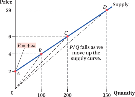
As we move up along the supply curve, the P/Q ratio falls. It’s probably obvious that it must fall from infinity, but you might wonder whether it keeps falling, because both P and Q are rising. It turns out that, yes, it must keep falling. The way to see this is to recognize that the P/Q ratio at any point on the supply curve equals the slope of a ray from the origin to that point. (The rise of the ray is the price P, and its run is the quantity Q. Because slope is rise over run, the ray’s slope is P/Q.) We’ve drawn some examples of such rays for different locations on the supply curve in Figure 2.16. It’s clear from the figure that as we move up and to the right along the supply curve, the slopes of these rays from the origin continue to fall.
46
Unlike with the demand curve, however, the P/Q ratio never falls to zero because the supply curve will never intercept the horizontal axis. Therefore, the price elasticity of supply won’t drop to zero. In fact, while the P/Q ratio is always falling as we move up along the supply curve, you can see from the figure that it will never drop below the slope of the supply curve itself. Some linear supply curves like the one in Figure 2.16 intercept the vertical axis at a positive price, indicating that the price has to be at least as high as the intercept for producers to be willing to supply any positive quantity. Because the price elasticity of supply equals (1/slope) × (P/Q), such supply curves approach becoming unit elastic at high prices and quantities supplied, but never quite get there. Also, because P/Q never falls to zero, the only way a supply curve can have an elasticity of zero is if its inverse slope is zero—
 See the problem worked out using calculus
figure it out 2.5
The demand for gym memberships in a small rural community is Q = 360 – 2P, where Q is the number of monthly members and P is the monthly membership rate.
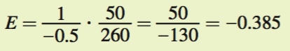
Calculate the price elasticity of demand for gym memberships when the price is $50 per month.
Calculate the price elasticity of demand for gym memberships when the price is $100 per month.
Based on your answers to (a) and (b), what can you tell about the relationship between price and the price elasticity of demand along a linear demand curve?
Solution:
The price elasticity of demand is calculated as
Let’s first calculate the slope of the demand curve. The easiest way to do this is to rearrange the equation in terms of P to find the inverse demand curve:
Q = 360 – 2P
2P = 360 – Q
P = 180 – 0.5Q
We can see that the slope of this demand curve is –0.5. We know this because every time Q rises by 1, P falls by 0.5.
So we know the slope and the price. To compute the elasticity, we need to know the quantity demanded at a price of $50. To find this, we plug $50 into the demand equation for P:
Q = 360 – 2P = 360 – 2(50) = 360 – 100 = 260
Now we are ready to compute the elasticity:
When the price is $100 per month, the quantity demanded is
Q = 360 – 2P = 360 – 2(100) = 360 – 200 = 160
Plugging into the elasticity formula, we get
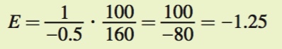
From (a) and (b), we can see that as the price rises along a linear demand curve, demand moves from being inelastic (|–0.385| < 1) to elastic (|–1.25| > 1).
Perfectly Inelastic and Perfectly Elastic Demand and Supply
The formula relating elasticities to slopes also sheds some light on what demand and supply curves look like in two special but often discussed cases: perfectly inelastic and perfectly elastic demand and supply.
47
Perfectly Inelastic We discussed above that when the price elasticity is zero, demand and supply are said to be perfectly inelastic. We just saw that this will be true for any linear demand at the point where it intercepts the horizontal (quantity) axis. But what would a demand curve look like that is perfectly inelastic everywhere? A linear demand curve with a slope of –∞ would drive the price elasticity of demand to zero due to the inverse relationship between elasticity and slope. Because a curve with an infinite slope is vertical, a perfectly inelastic demand curve is vertical. An example of such a curve is shown in Figure 2.17a. This makes intuitive sense: A vertical demand curve indicates that the quantity demanded by consumers is completely unchanged regardless of the price. Any percentage change in price will induce a 0% change in quantity demanded. In other words, the price elasticity of demand is zero.
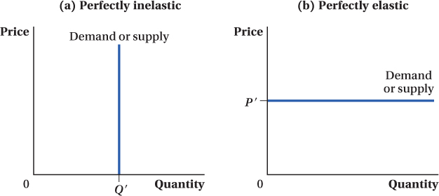
While perfectly inelastic demand curves don’t really exist (after all, there are almost always possibilities for consumers and producers to substitute toward or away from a good as prices hit either extreme of zero or infinity), we might see some situations approaching them. For example, diabetics might have very inelastic demand for insulin. Their demand curve will be almost vertical if they will buy it at any price.
The same logic holds for supply: A vertical supply curve indicates perfectly inelastic supply and no response of quantity supplied to price differences. The supply of tickets for a particular concert or sporting event might also be close to perfectly inelastic, with a near-
One implication of perfect inelasticity is that any shift in the market’s demand or supply curve will result in a change only in the market equilibrium price, not the quantity. That’s because there is absolutely no scope for quantity to change in the movement along a perfectly inelastic demand curve from the old to the new equilibrium. Likewise, for perfectly inelastic supply, if there is a demand curve shift, all equilibrium movement is in price, not quantity.
Perfectly Elastic When demand or supply is perfectly elastic, on the other hand, the price elasticity is infinite. This will be the case for linear demand or supply curves that have slopes of zero—
48
Small producers of commodity goods probably face demand curves for their products that are approximately horizontal. (We’ll discuss this more in Chapter 8.) For instance, a small corn farmer can probably sell as many bushels of corn as she wants at the market price. If the farmer decided that the price was too low and insisted that she be paid more than the going rate, no one would buy her corn. They could buy from someone else for less. Effectively, then, it is as if the farmer faces an infinite quantity demanded for her corn at the going price (or below it, if for some reason she’s willing to sell for less) but zero quantity demanded of her corn above that price. In other words, she faces a flat demand curve at the going market price.
Supply curves are close to perfectly elastic in competitive industries in which producers all have roughly the same costs, and entry and exit are very easy. (We’ll also discuss this point at greater length in Chapter 8.) These conditions mean that competition will drive prices toward the (common) level of costs, and differences in quantities supplied will be soaked up by the entry and exit of firms from the industry. Because of the strictures of competition in the market, no firm will be able to sell at a price above costs, and obviously no firm will be willing to supply at a price below costs. Therefore, the industry’s supply curve is essentially flat at the producers’ cost level.
As opposed to the perfectly inelastic case, shifts in supply in a market with perfectly elastic demand will only move equilibrium quantity, not price. There’s no way for the equilibrium price to change when the demand curve is flat. Similarly, for markets with perfectly elastic supply, demand curve shifts move only equilibrium quantities and not prices.
Income Elasticity of Demand
We’ve been focusing on price elasticities to this point, and with good reason: They are a key determinant of demand and supply behavior and play an important role in helping us understand how markets work. However, they are not the only elasticities that matter in demand and supply analysis. Remember how we divided up all the factors that affected demand or supply into two categories: price and everything else? Well, each of those other factors that went into “everything else” has an influence on demand or supply that can be measured with an elasticity.
The most commonly used of these elasticities measure the impact of two other factors on quantity demanded. These are the income elasticity of demand and the cross-
income elasticity of demand
The percentage change in quantity demanded associated with a 1% change in consumer income.
The income elasticity of demand is the ratio of the percentage change in quantity demanded to the corresponding percentage change in consumer income (I):
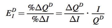
(Equivalently, it is the percentage change in quantity demanded associated with a 1% change in consumer income.)
49
inferior good
A good for which quantity demanded decreases when income rises.
Income elasticities describe how responsive demand is to income changes. Goods are sometimes categorized by the sign and size of their income elasticity. Goods that have an income elasticity that is negative, meaning consumers demand a lower quantity of the good when their income rises, are called inferior goods. This name isn’t a comment on their inherent quality; it just describes how their consumption changes with people’s incomes. (Note, however, that low-
normal good
A good for which quantity demanded rises when income rises.
Goods with positive income elasticities (consumers’ quantity demanded rises with their income) are called normal goods. As the name indicates, most goods fit into this category.
luxury good
A good with an income elasticity greater than 1.
Normal goods with income elasticities above 1 are sometimes called luxury goods. Having an income elasticity that is greater than 1 means the quantity demanded of these products rises at a faster rate than income. As a consequence, the share of a consumer’s budget that is spent on a luxury good becomes larger as the consumer’s income rises. (To keep a good’s share of the budget constant, quantity consumed would have to rise at the same rate as income. Because luxury goods’ quantities rise faster, their share increases with income.) Yachts, butlers, and fine art are all luxury goods.
Cross-Price Elasticity of Demand
cross-
The percentage change in the quantity demanded of one good associated with a 1% change in the price of another good.
The cross-
own-
The percentage change in quantity demanded for a good resulting from a percentage change in the price of that good.
(To avoid confusion, sometimes the price elasticities we discussed above, which are concerned with the percentage change in quantity demanded to the percentage change in the price of the same good, are referred to as own-
When a good has a positive cross-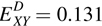 and 0.149, respectively). However, it is much less of a substitute for the more adult Shredded Wheat, which had a cross-
When a good has a negative cross-
50
figure it out 2.6
Suppose that the price elasticity of demand for cereal is –0.75 and the cross-
Solution:
The first step will be to see what happens to the quantity of cereal demanded when the price of milk rises by 10%. We can use the cross-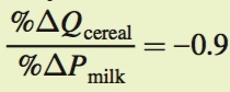 Using the equation, we know that the denominator is 10 since the price of milk rose by 10%, so we get
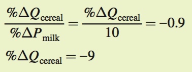
Thus, when the price of milk rises by 10%, the quantity demanded of cereal falls by 9%.
Now we must consider how to offset this decline in the quantity of cereal demanded with a change in the price of cereal. In other words, what must happen to the price of cereal to cause the quantity of cereal demanded to rise by 9%? It is clear that the price of cereal must fall because the law of demand suggests that there is an inverse relationship between price and quantity demanded. However, because we know the price elasticity of demand, we can actually determine how far the price of cereal needs to fall.
The price elasticity of demand for cereal is
To offset the decline in cereal consumption caused by the rise in the price of milk, we need the percentage change in quantity demanded to be +9%. Therefore, we can plug 9% into the numerator of the ratio and solve for the denominator:
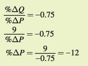
The price of cereal would have to fall by 12% to exactly offset the effect of a rise in the price of milk on the quantity of cereal consumed.