Politicians call regularly for price ceilings on products whose prices have risen a lot. In this section, we explore the effects of direct government interventions in market pricing. We look both at regulations that set maximum prices (like a gas price ceiling) and minimum prices (price floors like a minimum wage).

71

A price ceiling establishes the highest price that can be paid legally for a good or service. At various times, regulations have set price ceilings for cable television, auto insurance, flood insurance, electricity, telephone rates, gasoline, prescription drugs, apartments, food products, and many other goods.

To look at the impact of a price ceiling, let’s suppose the city council of a college town passes a pizza price control regulation. With the intent of helping out the college’s financially strapped students, the city council says no pizzeria can charge more than $8 for a pizza. Let’s say the demand curve for pizzas in a month during the school year is described by the equation Q^D = 20,000 – 1,000P. The cheaper pizzas get, the more students will eat them, so the demand curve slopes downward. If the price were zero, 20,000 pizzas would be sold per month (it’s not that big a college, and there are only so many meals one can eat). The demand choke price is $20 per pizza—if the price were $20 per pizza, no pizzas would be sold.

Let’s say the supply of pizzas is given by Q^S = 2,000P – 10,000. Supply slopes upward because when prices are higher, the pizzerias make more pizzas. If the price is below $5, they make no pizzas. For each $1 increase in the price of a pizza after that, an additional 2,000 pizzas per month would be supplied.

Figure 3.7 graphs the supply and demand curves described by these two equations. It shows that the free-market equilibrium is at point w; that is, before price controls, the equilibrium price for a pizza is $10, and at that price, 10,000 pizzas are supplied and demanded. Given these baseline market conditions, we can study the impact of the price ceiling using the graph or the equations. Let’s start with the graph.

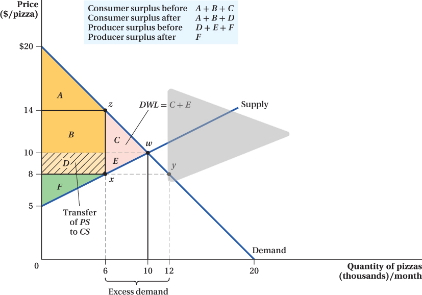
Graphical Analysis Before any price controls, the consumer surplus for pizza-eating students is given by the area below the demand curve and above the $10 free-market price, A + B + C. The producer surplus is the area above the supply curve but below the price, D + E + F.

When the city council implements the price control regulation, the highest price the pizzerias can charge is $8 per pizza, which is less than the market-clearing price of $10. At $8, students demand a total of 12,000 pizzas (point y). This quantity demanded is larger than the 10,000 pizzas demanded at the free-market equilibrium because the price ceiling price is lower than the free-market price. At an $8 price, however, pizzerias are only willing to supply 6,000 pizzas. That is, there is excess demand: The quantity demanded exceeds the quantity supplied at that price. There will be a large number of students frustrated that they cannot buy the number of pizzas they would like at the price ceiling.

Now let’s consider how the price ceiling affects consumer and producer surplus. It’s clear that the pizzerias are worse off. In the free market, they would have sold more pizzas (10,000 versus 6,000) at a higher price ($10 versus $8). The producer surplus after the price control law is everything below the capped price and above the supply curve; producer surplus shrinks from area D + E + F to area F.

The law was passed to benefit students by lowering pizza prices. But we can’t actually say for sure whether they are better off as a result. The analysis of consumer surplus can become a bit complicated in situations with excess demand. Excess demand can create incentives for buyers to come into the market who wouldn’t have even been interested in the product if not for the price ceiling, because these buyers hope to obtain the good at the low, controlled price and resell it to high-value buyers at a higher price. (This is why ticket brokers who have no interest in seeing a sold-out concert or game still try hard to obtain tickets to it.) How many such buyers come into the market, what they eventually resell the good for, and any additional costs of this reselling process all affect how much surplus is in the market and who obtains it. Here, we analyze what in some sense is the best-case scenario when there is excess demand: Suppliers directly sell what they are willing to sell at the price ceiling to those consumers with the highest valuation for those limited units of the good. Even under this best-case scenario, there is no guarantee that the ceiling makes consumers better off overall.

72

The consumer surplus with the price ceiling is the area below the demand curve and above the price, area A + B + D. The consumer surplus now includes area D because the price is lower. We call area D a transfer from producers to consumers, because imposing price controls shifted that area from being part of producer surplus to being part of consumer surplus. However, fewer pizzas are bought after the price cap law, resulting in consumers losing area C. Therefore, the net impact of the price cap on consumers depends on the relative sizes of the surplus transferred from the producers (area D) and loss reflected in area C. For those students who are able to buy the 6,000 pizzas in a month at a price that is $2 lower than they did before the law was enacted, life is good. They are the ones to whom area D is transferred. But for the students who would have enjoyed 4,000 more pizzas in the free market that they can no longer buy, life is a hungry proposition.

73

The producer surplus and consumer surplus represented by areas C and E have disappeared because of the price ceiling. No one receives these surpluses anymore. Their combined areas are known as a deadweight loss (DWL). Deadweight loss is the difference between the maximum total surplus that consumers and producers could gain from a market and the combined gains they actually reap after a price regulation, and it reflects the inefficiency of the price ceiling. It’s called a deadweight loss because it represents a set of mutually beneficial, surplus-generating transactions (pizza purchases, in this case) that would have occurred in an unregulated market with a customer who was willing to buy and a producer who was willing to sell at the market price. Area C is the deadweight loss suffered by consumers; area E is lost by producers.

Why is there a loss in consumer surplus if the students get to keep the money that they’re not spending on pizza? Remember, the students missing out on the 4,000 pizzas after the price control law don’t want to save the $10—they want the pizza! The reason a loss of consumer surplus occurs is that the pizzas those students would have gotten in a market without a price control would be worth more than $10 to them. People who buy are on the part of the demand curve that is above the market price (except that individual right at the market price); their willingness to pay is greater than the price they have to pay. The price control results in their losing that difference.

Some producer surplus also becomes deadweight loss as a result of the price ceiling. There are pizzerias that would be willing to sell pizzas for more than $8 but less than the $10 equilibrium price. Once the $8 price ceiling is in place, pizzerias will pull 4,000 pizzas off the market because $8 is not enough to cover their costs of making those extra pizzas. So both students and pizzerias were benefiting from transactions that took place before the price control; once the price ceiling is imposed, however, some of those transactions no longer take place and these benefits are lost.

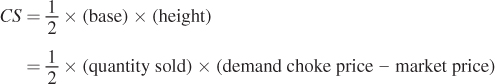
Analysis Using Equations Now let’s compare the free and regulated markets for pizzas using the supply and demand equations we described earlier. To determine the free-market equilibrium using the equations, we set quantity supplied equal to quantity demanded and solve for the market clearing price P:

Q^S = Q^D

2,000P – 10,000 = 20,000 – 1,000P

3,000P = 30,000

P = $10

Plugging that price back into either the supply or demand equation gives an equilibrium quantity of 10,000 pizzas:

The consumer surplus in the free market is the triangle A + B + C. The area of that triangle is

74

The demand choke price is the price at which Q^D = 0. In this case,

0 = 20,000 – 1,000(P_DChoke)

1,000(P_DChoke) = 20,000

(P_DChoke) = $20

The consumer surplus triangle is

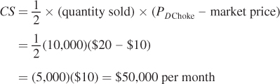
(Remember that quantities are measured in pizzas per month, so the consumer surplus is measured in dollars per month.)

The producer surplus is the triangle D + E + F in the graph. The area of that triangle is

The supply choke price is the price at which quantity supplied is zero:

Q^S = 2,000P – 10,000

0 = 2,000(P_SChoke) – 10,000

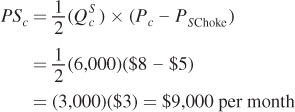
P_SChoke = 10,000/2,000 = $5

Plugging this price into the equation for producer surplus, we find

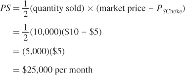
Now let’s consider the impact of the price ceiling. The price of a pizza cannot rise to $10 as it did in the free market. The highest it can go is $8. We saw in the graphical analysis that this policy led to excess demand, the difference between the quantity demanded and the quantity supplied at the price ceiling (P_c):

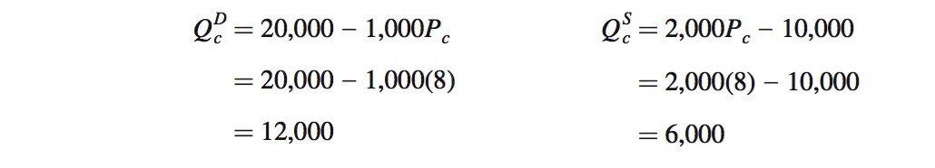
The excess demand is 12,000 – 6,000 or 6,000 pizzas per month. This means that there are students ringing pizzerias’ phones off the hook trying to order more pizzas, but whose orders the pizzerias won’t be willing to fill at the new market price.

Next, we compute the consumer and producer surpluses after the price control is imposed. Producer surplus is area F:

75

which is just over one-third of the $25,000 of producer surplus pizzerias were making before the price ceiling. It is no wonder that producers fight against laws like this one.

The consumer surplus is now areas A + B + D. An easy way to figure out the value for this surplus is to add the area of triangle A to the area of the rectangles B and D. Triangle A has an area of

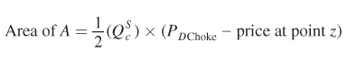
where the price at point z is the price at which quantity demanded equals the new quantity supplied of 6,000 pizzas. To determine this price, set Q^D = Q_c^S and solve for the price:

Q^D = 20,000 – 1,000P_z = Q_c^S

20,000 – 1,000P_z = 6,000

20,000 – 6,000 = 1,000P_z

P_z = 14,000/1,000 = $14

This means that, if the price of a pizza were actually $14, exactly 6,000 pizzas would be demanded. With this value for the price at point z, we can now calculate:

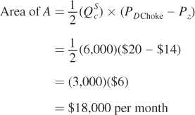
The area of rectangle B is

B = Q_c^S × (P_z – free-market price)

= (6,000)($14 – $10)

= $24,000 per month

and the rectangle D is

D = Q_c^S × (free-market price – P_c)

= (6,000)($10 – $8)

= $12,000 per month

Adding these three areas, we find that total consumer surplus after the pizza price ceiling is A + B + D = $54,000 per month.

Therefore, consumers as a group are better off than they were under the free market: They have $4,000 more of consumer surplus per month. However, this outcome hides a big discrepancy. Those students lucky enough to get in on the 6,000 pizzas for $8 rather than $10 are better off, but there are 4,000 pizzas that would have been available in the free market that are no longer being supplied. Students who would have consumed those missing pizzas are worse off than they were before.

76

What is the deadweight loss from the inefficiency of this price-controlled market outcome? The full DWL is the area of triangle C + E in the figure, so

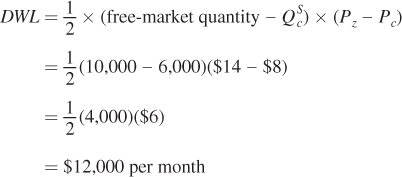
The Problem of Deadweight Loss As we have seen, a price ceiling creates a deadweight loss. This deadweight loss is just that: lost. It’s surplus that was formerly earned by consumers (C ) or producers (E ) that neither gets when there is a price ceiling. This analysis has shown that price ceilings and other mandates and regulations can come with a cost, even if they don’t involve any direct payments from consumers or producers (as taxes do).

A natural way to think about the size of the deadweight loss is as a share of the transfer D. Because the price control was designed to transfer surplus from pizzerias to students, the deadweight loss tells us how much money gets burned up in the process of transferring surplus through this regulation. In this case, the deadweight loss ($12,000) is just as large as the transfer. In other words, in the process of transferring income from pizzerias to students through the price ceiling, one dollar of surplus is destroyed for every dollar transferred.

This example illustrates the dilemma of using regulations to transfer income. If somehow the city council could get the producers to directly pay the consumers the amount D – C without changing the price, the consumers would be just as happy as with the price control, because that’s all they net in the deal after losing the deadweight loss. The producers would be better off as well. Rather than being left with just F, they would have their free-market producer surplus of D + E + F minus their payment of D – C. The areas D in these two values cancel, leaving the pizzerias E + F + C, which is larger than the F in producer surplus they get under the price ceiling law. Deadweight loss occurs because the price-control regulation transfers income by changing prices, and price changes affect incentives and lead to inefficiency. Practically speaking, though, it’s difficult to figure out how to organize the payment of D – C without changing the price. A per pizza subsidy paid by pizzerias to students, for example, would have the same result as reducing the price and would thus have its own deadweight loss as we describe in Section 3.5.

Importance of Price Elasticities The elasticities of supply and demand are the keys to the relative sizes of the deadweight loss and the transfer. Consider two different pizza markets in Figure 3.8. In panel a, the curves are relatively inelastic and show little price sensitivity. In panel b, the relatively elastic supply and demand curves reflect a greater amount of price sensitivity. 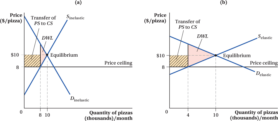It’s clear from the figure that if the same price-control rule is applied to both markets, the deadweight loss will be larger as a share of the transfer in the market with more elastic supply and demand.

The intuition behind this result is that the price ceiling’s deadweight loss comes about because it keeps a set of sellers and buyers who would be willing to trade in the market at the free-market price from doing so. If the number of people in this set is small (in other words, the quantity after the regulation is close to the quantity before), then the deadweight distortion is small. How large that number of people is depends on how sensitive supply and demand are to prices. If supply and demand are relatively inelastic, the number of people and firms changing their quantity demanded or supplied will be small, and the DWL will be small relative to the transfer. If supply and demand are relatively elastic, the number of people and firms who change their quantity demanded or supplied will be large.

77

Nonbinding Price Ceilings In the pizza example, the price ceiling was below the free-market equilibrium price. What if a ceiling were set above the equilibrium price? Suppose the city council passed a law that limited the price of pizzas to $12 instead of $8, for example.

In such cases, the price ceiling has no effect. Because it is set at a level above where the market would clear anyway ($10 in the pizza case), it won’t distort market outcomes. There will be no impact on price, no excess demand, and no deadweight loss. Price ceilings at levels above the equilibrium price are said to be nonbinding, because they do not bind or keep the market from arriving at its free-market outcome.

The other major type of price regulation is a price floor (sometimes called a price support), a limit on how low a product’s price can go. Lawmakers around the world use price floors to prop up the prices of all sorts of goods and services. Agricultural products are a favorite. In the United States, the federal government began setting price supports for agricultural goods such as milk, corn, wheat, tobacco, and peanuts as early as the 1930s. The goal was to guarantee farmers a minimum price for their crops to protect them from fluctuating prices. Many of these price supports remain today. We will use the tools of consumer and producer surplus to analyze price floors just as we used them for price ceilings.

78

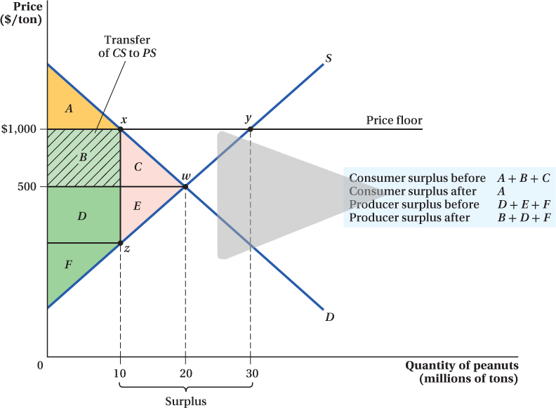
Let’s look at the market for peanuts. The unregulated market for peanuts is shown in Figure 3.9. The equilibrium quantity of peanuts is 20 million tons, and the equilibrium price of peanuts is $500 per ton. The government decides that farmers should be getting more than $500 per ton for their peanuts, so it passes a regulation that peanuts must sell for no less than $1,000 per ton.

Immediately, we know there is going to be a problem. At the higher price, peanut farmers want to sell lots of peanuts—30 million tons. But at that price, quantity demanded is much lower—only 10 million tons. (Peanut butter sandwiches are just too expensive when peanuts cost $1,000 per ton.) This imbalance leads to excess supply in the market: Sellers want to sell more of the product at that price than buyers want to buy. This is indicated in the figure by the 20-million-ton difference between the quantity of peanuts supplied and the quantity demanded at the price floor.

79

The goal of the price floor policy is to help farmers, so we need to look at the producer surplus to know how well the policy accomplishes its goal. Before the regulation, producer surplus was the area D + E + F. After the regulation, prices go up for all the peanut farmers who are still able to find buyers, so producers gain area B as a transfer from consumers. The farmers sell 10 million tons of peanuts and receive $500 per ton more than they were receiving in the free market. But peanut growers lose some of their market. The reduction in quantity demanded from 20 million to 10 million tons knocks out producers who used to sell peanuts at market prices and made a small amount of producer surplus from it. This area E then becomes the producers’ part of the deadweight loss (DWL) from the regulation.

Overall, the producers gain surplus of B – E. If supply and demand are sufficiently elastic (i.e., if both curves are flat enough), producers could actually be made worse off from the price floor that was put in place to help them. This is because area E—the producers’ share of the DWL—may be larger than the transfer from consumers, area B. This outcome is another application of our discussion above about how the deadweight loss grows as the supply and demand curves become more elastic.

How do consumers fare when the price floor is enacted? You can probably guess: Consumer surplus falls from A + B + C to A. Area B is the surplus transferred from consumers to producers, and area C is the consumer part of the DWL.

The price floor policy therefore transfers income from consumers to peanut farmers, but only by burning C + E (the DWL) to do it. Again, if there were some way for the consumers to directly pay the peanut farmers a set amount equal to area B, the farmers would obtain more surplus than they get with the regulation (producer surplus of B versus B – E ), and the consumers would be better off too (consumer surplus of A + C instead of A). By changing the actual price of peanuts instead of making a transfer unrelated to quantity, the price support distorts people’s incentives and leads to inefficiency, as reflected by the DWL of C + E.

This analysis also illustrates the everlasting dilemma of price supports. The quantity supplied at the price floor is greater than the quantity demanded. So what happens to the extra peanuts? They accumulate in containers rather than being sold on the market. To avoid this outcome, a government will often pay the producers who can’t sell their output in the regulated market to stop producing the extra output (20 million extra tons of peanuts in our example). The United States Department of Agriculture, for example, oversees various programs to reduce the surplus of price-supported crops on the market. One such program, the Conservation Reserve Program (CRP), paid farmers $1.90 billion in 2014 (an average of about $64 per acre) for holding land out of production. The program does have environmental benefits that mitigate some of the losses, but it also serves to reduce the quantity of subsidized crops that is grown, effectively by replacing those subsidies with CRP payments. There are also a number of programs that distribute billions of dollars annually ($2 billion in 2014) of commodity foods—like peanut butter—to school lunch programs and needy individuals on the condition that the foods not be resold. Again, these programs take surplus crops off the market.

Another example of a price support is a minimum wage. Here, the “product” is labor and the “price” is the wage, but the analysis is the same. If the government tries to help college students save tuition money by mandating that all summer internships pay at least $40 an hour, the quantity of labor supplied for internships will be much greater than the quantity demanded. As a result, there will be a lot of unemployed intern-hopefuls who would have been working at the equilibrium wage.

Just as with our earlier examples, how many people a minimum wage adds to the number of unemployed (the excess quantity supplied in the price floor figure), the amount of income transferred to workers (the change in producer surplus), and the size of the deadweight loss all depend on the elasticity of labor supply and labor demand. The price floor’s deadweight loss arises because a set of sellers and buyers who would be willing to trade in the market at the free-market price will not do so at the regulated price. When suppliers and demanders are relatively insensitive to price, the number of transactions that the price floor prevents from happening is relatively small, and therefore so is the deadweight loss. Large price elasticities imply a large number of destroyed transactions and a large deadweight loss relative to the transfer of income.

80

Nonbinding Price Floors If a price floor is set below the free-market equilibrium price, it will have no effect on the market. This would be the case if, for example, the peanut price floor had been set at $400, below the equilibrium price of $500. Nonbinding price floors have no effect on price and do not create excess supply or deadweight loss.