5.3 Decomposing Consumer Responses to Price Changes into Income and Substitution Effects
When the price of a good changes, the demand curve for that good tells us how much consumption will change. This total change in quantity demanded, however, is a result of two distinct forces that affect consumers’ decisions: the substitution effect and the income effect. Any change in quantity demanded can be decomposed into these two effects.
substitution effect
The change in a consumer’s consumption choices that results from a change in the relative prices of two goods.
When the price of one good changes relative to the price of another good, consumers will want to buy more of the good that has become relatively cheaper and less of the good that is now relatively more expensive. Economists call this the substitution effect.
income effect
The change in a consumer’s consumption choices that results from a change in the purchasing power of the consumer’s income.
A price shift changes the purchasing power of consumers’ incomes—
the amount of goods they can buy with a given dollar- level expenditure. If a good gets cheaper, for example, consumers are effectively richer and can buy more of the cheaper good and other goods. If a good’s price increases, the purchasing power of consumers’ incomes is reduced, and they can buy fewer goods. Economists refer to consumption changes resulting from this shift in spending power as the income effect.
170
Any change in quantity demanded can be decomposed into these two effects. We introduce them in this book, but we are just scratching the surface. We’re going to be upfront with you: The distinction between income and substitution effects is one of the most subtle concepts that you will come across in this entire book. If you go on to take more advanced economics courses, income and substitution effects will come up again and again.3 Two factors make this topic difficult. First, we never separately observe these two effects in the real world, only their combined effects. Their separation is an artificial analytical tool. Put another way, as a consumer, you can (and do) figure out how much to consume without knowing or figuring out how much of the change is due to income effects and how much is due to substitution effects. Second, the income effect occurs even when the consumer’s income as measured in dollars remains constant. How rich we feel is determined both by how much income we have and how much things cost. If your income stays at $1,000 but the prices of all goods fall by half, you are effectively a lot wealthier. The income effect refers to how rich you feel, not the number of dollar bills in your pocket.
In our overview, we demonstrate income and substitution effects using graphs. The appendix to this chapter describes these effects mathematically.
total effect
The total change (substitution effect + income effect) in a consumer’s optimal consumption bundle as a result of a price change.
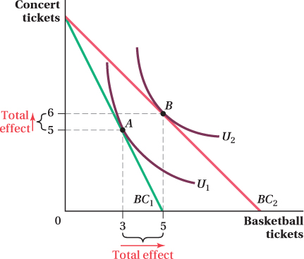
Figure 5.9 shows how one consumer, Carlos, who spends his income on attending music concerts and basketball games, reacts to a fall in the price of basketball tickets. This is just like the analysis we did in Section 5.2. If basketball ticket prices fall, the budget constraint rotates outward from BC1 to BC2 because Carlos can now purchase more basketball tickets with his income. As a result, the optimal consumption bundle shifts from A (the point of tangency between indifference curve U1 and budget constraint BC1) to B (the point of tangency between indifference curve U2 and budget constraint BC2). Because of the fall in the price of basketball tickets, the quantity of concert tickets consumed increases from 5 to 6, and the number of basketball tickets Carlos purchases rises from 3 to 5. These overall changes in quantities consumed between bundles A and B are the total effect of the price change.
171
Note that just as in Section 5.2, we figured out the optimal bundle without any reference to income or substitution effects. In the next sections, we decompose the total effect into separate substitution and income effects. That is,
Total Effect = Substitution Effect + Income Effect
Breaking down the movement from A to B into income and substitution effects helps us understand how much of the total change in Carlos’s quantity demanded occurs because Carlos switches what he purchases as a result of the reduction in the relative prices of the two goods (the substitution effect), and how much of the change is driven by the fact that the decrease in the price of basketball tickets gives Carlos more purchasing power (the income effect).
Note also that all the examples we work through involve a drop in the price of a good. When the price of a good increases, the effects work in the opposite direction.
Isolating the Substitution Effect
Let’s begin by isolating the substitution effect. This part of the change in quantities demanded is due only to the change in relative prices, not to the change in Carlos’s buying power. To isolate the substitution effect, we need to figure out how many concert and basketball tickets Carlos would want to buy if, after the price change, there was no income effect, that is, if he had the same purchasing power as before the price change and felt neither richer nor poorer.
For Carlos to feel neither richer nor poorer, the bundle he consumes after the price change must provide him with the same utility he was receiving before the price change; that is, the new bundle must be on the initial indifference curve U1.
The substitution-
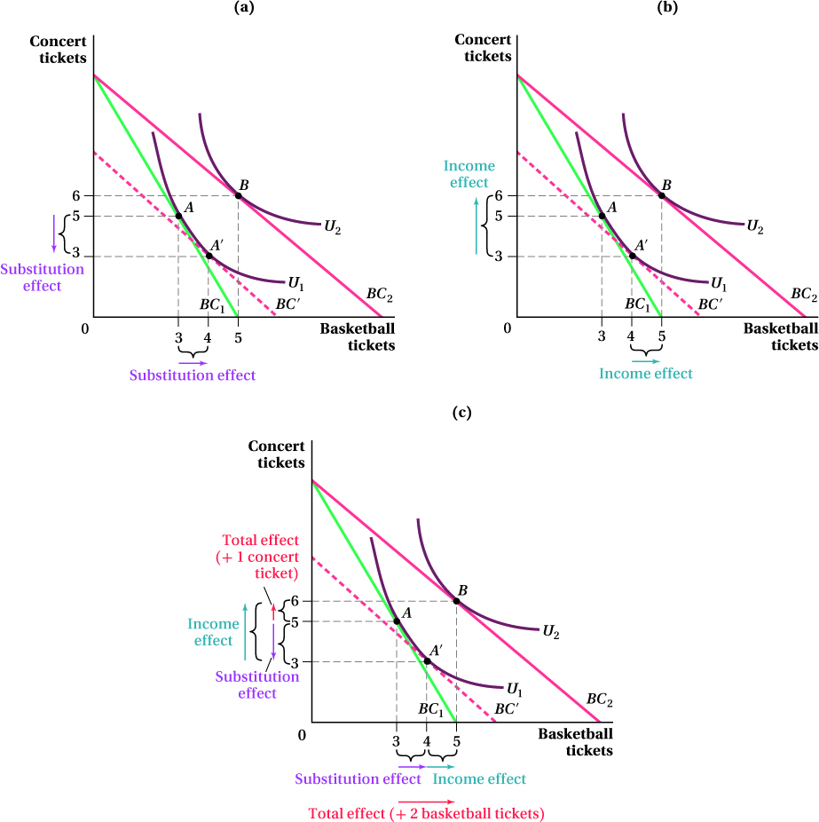
Bundle A′ is what Carlos would buy if the relative prices of concert and basketball tickets changed the same way, but Carlos experienced no change in purchasing power. This is the definition of the substitution effect. Thus, the substitution effect, in isolation, moves Carlos’s demanded bundle from A to A′. To find this effect, we have to shift the postprice-
There are a few things to notice about the change in quantities due to the substitution effect. First, the quantity of concert tickets decreases (from 5 to 3), and the quantity of basketball tickets increases (from 3 to 4). The decrease in the quantity of concert tickets demanded occurs because the price change has caused basketball tickets to become cheaper relative to concert tickets, so Carlos wants to buy relatively more basketball tickets. Second, while points A and A′ are on the same indifference curve (and Carlos therefore gets the same utility from either bundle), it costs Carlos less to buy bundle A′ at the new prices than to buy A. We know this because point A is located above BC′ and so is infeasible if the budget constraint is BC′. (A′, however, being on BC′, is feasible with this constraint.)
172
173
Carlos therefore responds to the decline in basketball ticket prices by substituting away from concert tickets and toward basketball tickets. By moving down along U1, Carlos has effectively made himself better off; he is getting the same utility (he’s still on U1) for less money (bundle A is no longer feasible even though A′ is).
Isolating the Income Effect
The income effect is the part of the total change in quantities consumed that is due to the change in Carlos’s buying power after the price change. Why is there an income effect even though only the price of a good changed, not the actual number of dollars that Carlos had to spend? The key to understanding this outcome is to recognize that when the price of a good falls, Carlos becomes richer overall. The reduction in a good’s price means there’s a whole new set of bundles Carlos can now buy that he couldn’t afford before because he has more money left over. At the old prices, everything above and to the right of BC1 was infeasible; at the new prices, only bundles outside BC2 are infeasible (see panel b of Figure 5.10).
This increase in buying power allows Carlos to achieve a higher level of utility than he did before. The income effect is the change in Carlos’s choices driven by this shift in buying power while holding relative prices fixed at their new level. Finding these income-
Therefore, the income effect of the decline in the basketball ticket price is illustrated by the move from the substitution-
In this particular example, the income effect led to increases in the quantities of both concert and basketball tickets. That means both goods are normal goods. In the next section, we show an example in which one of the goods is inferior.
The Total Effects
The total effects of the decline in basketball ticket prices are shown in panel c of Figure 5.10:
The quantity of concert tickets Carlos desires rises by 1 ticket from 5 in the initial bundle at point A to 6 in the final bundle at point B. (A decline of 2 caused by the substitution effect is counteracted by a rise of 3 caused by the income effect for a net gain of 1 concert ticket.)
The quantity of basketball tickets Carlos wants to buy rises by 2, from 3 in the initial bundle A to 5 in the final bundle B. (A rise of 1 caused by the substitution effect plus a rise of 1 caused by the income effect.)
174
make the grade
Computing substitution and income effects from a price change
There are three basic steps to analyzing substitution and income effects. We start with the consumer at a point of maximum utility (Point A) where his indifference curve is tangent to his budget constraint.
When prices change, draw the new budget constraint (a price change rotates the budget constraint, altering its slope).Then find the optimal quantity at the point (Point B) where this new budget constraint is tangent to a new indifference curve.
Draw a new line that is parallel to the new budget constraint from Step 1 and tangent to the original indifference curve at Point A′. The movement along the original indifference curve from Point A (the original, pre-
price change bundle) to this new tangency (point A′) is the substitution effect. This movement shows how quantities change when relative prices change, even when the purchasing power of income is constant. The income effect of the price change is seen in the movement from point A′ to point B. Here, relative prices are held constant (the budget lines are parallel) but the purchasing power of income changes.
What Determines the Size of the Substitution and Income Effects?
The size (and as we’ll see shortly, sometimes the direction) of the total effect of a price change depends on the relative sizes of its substitution and income effects. So it’s important to understand what factors influence how large substitution and income effects are. We discuss some of the more important factors below.
The Size of the Substitution Effect The size of the substitution effect depends on the degree of curvature of the indifference curves. You can see this in Figure 5.11. The figure’s two panels show the substitution effects of the same change in the relative prices of concert and basketball tickets for two different indifference curve shapes. (We know it’s the same relative price change because the budget constraints’ slope changes by the same amount in both panels.) When indifference curves are highly curved, as in panel a, the MRS changes quickly as one moves along them. This means any given price change won’t change consumption choices much, because one doesn’t need to move far along the indifference curve to change the MRS to match the new relative prices. Thus, the substitution effect is small. This is unsurprising, because we learned in Chapter 4 that indifference curves have more curvature when two goods are not highly substitutable. In panel a, the relative price change causes a substitution from A to A′, and the consumer moves from purchasing a bundle with 2 basketball tickets and 2 concert tickets to a bundle containing 3 basketball tickets and 1.25 concert tickets.
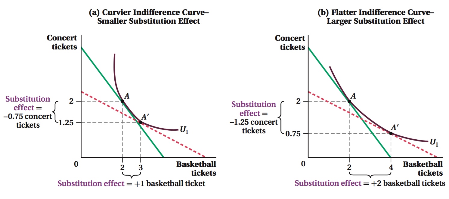
When indifference curves are less curved, as in panel b, the MRS doesn’t change much along the curve, so the same relative price change causes a much greater substitution effect. The substitution from A to A′ in panel b involves much larger changes in basketball and concert ticket consumption than that caused by the same relative price change in panel a.4 In panel b, the quantity of basketball game tickets purchased grows to 4 (rather than 3) and the quantity of music concert tickets purchased falls to 0.75 (rather than 1.25). Again, we can relate this to what we learned about the curvature of indifference curves in Chapter 4. Indifference curves with little curvature indicate that the two goods are close substitutes. Thus, it makes sense that a price change will lead to a much greater adjustment in the quantities in the consumer’s preferred bundle.
175
The Size of the Income Effect The size of the income effect is related to the quantity of each good the consumer purchases before the price change. The more the consumer was spending on the good before the price change, the greater the fraction of the consumer’s budget affected by the price change. A price drop of a good that the consumer is initially buying a lot of will leave him with more income left over than a price drop of a good with a small budget share (and a price increase will sap a greater share of the consumer’s income). For example, think of how a change in the prices of electricity and pest control affect a typical homeowner. A typical consumer spends much more of his budget on electricity. Therefore, a change in the price of electricity will affect his income and alter his purchases by more than a similar change in the price of pest control. (At the extreme, if the consumer currently purchases no pest control, a change in the price of pest control will have no income effect at all.)
176
 See the problem worked out using calculus
figure it out 5.3
For interactive, step-
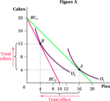
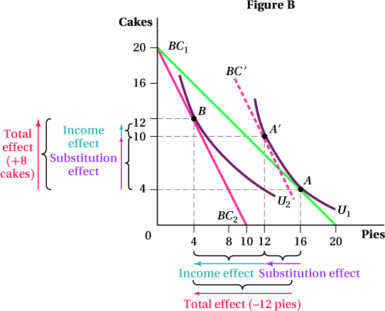
Pavlo eats cakes and pies. His income is $20, and when cakes and pies both cost $1, Pavlo consumes 4 cakes and 16 pies (point A in Figure A). But when the price of pies rises to $2, Pavlo consumes 12 cakes and 4 pies (point B).
Why does the budget constraint rotate as it does in response to the increase in the price of pies?
Trace the diagram on a piece of paper. On your diagram, separate the change in the consumption of pies into the substitution effect and the income effect. Which is larger?
Are pies a normal or inferior good? How do you know? Are cakes a normal or inferior good? How do you know?
Solution:
The price of cakes hasn’t changed, so Pavlo can still buy 20 cakes if he spends his $20 all on cakes (the y-intercept). However, at $2 per pie, Pavlo can now afford to buy only 10 pies instead of 20.
The substitution effect is measured by changing the ratio of the prices of the goods but holding utility constant (Figure B). Therefore, it must be measured along one indifference curve. To determine the substitution effect of a price change in pies, you need to shift the postprice-
change budget constraint BC2 out until it is tangent to Pavlo’s initial indifference curve U1. The easiest way to do this is to draw a new budget line BC′ that is parallel to the new budget constraint (thus changing the ratio of the cake and pie prices) but tangent to U1 (thus holding utility constant). Label the point of tangency A′. Point A′ is the bundle Pavlo would buy if the relative prices of cakes and pies changed as they did, but he experienced no change in purchasing power. When the price of pies rises, Pavlo would substitute away from buying pies and buy more cakes. The income effect is the part of the total change in quantities consumed that is due to the change in Pavlo’s buying power after the price of pies changes. This is reflected in the shift from point A′ on budget constraint BC′ to point B on budget constraint BC2. (These budget constraints are parallel because the income effect is measured holding relative prices constant.)
For pies, the income effect is larger than the substitution effect. The substitution effect leads Pavlo to purchase 4 fewer pies (from 16 to 12), while the income effect further reduces his consumption by 8 pies (from 12 to 4).
Pies are a normal good because Pavlo purchases fewer pies (4 instead of 12) when the purchasing power of his income falls due to the price increase. However, cakes are an inferior good because the fall in purchasing power actually leads to a rise in cake consumption.
177
An Example of the Income and Substitution Effects with an Inferior Good
Figure 5.12 provides another example of breaking out quantity changes into income and substitution effects. Here, however, one of the goods is inferior.
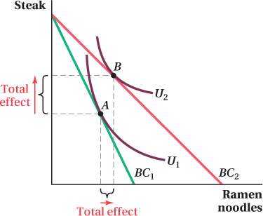
The graph shows Judi’s utility-
To split the shift from bundle A to bundle B into its substitution and income effects, we follow the steps we described in the previous section.
To find the substitution effect, we shift in the budget constraint after the price change until it is tangent to the original indifference curve U1. This is shown by the dashed line BC′ in panel a of Figure 5.13. The point of tangency between BC′ and U1 is bundle A′. Because this is the bundle that provides the same utility as the original bundle A but with ramen noodles at their new, lower price, the shift from A to A′ is the substitution effect. Just as before, the substitution effect leads Judi to consume more of the good that becomes relatively cheaper (ramen noodles) and less of the other good (steak).
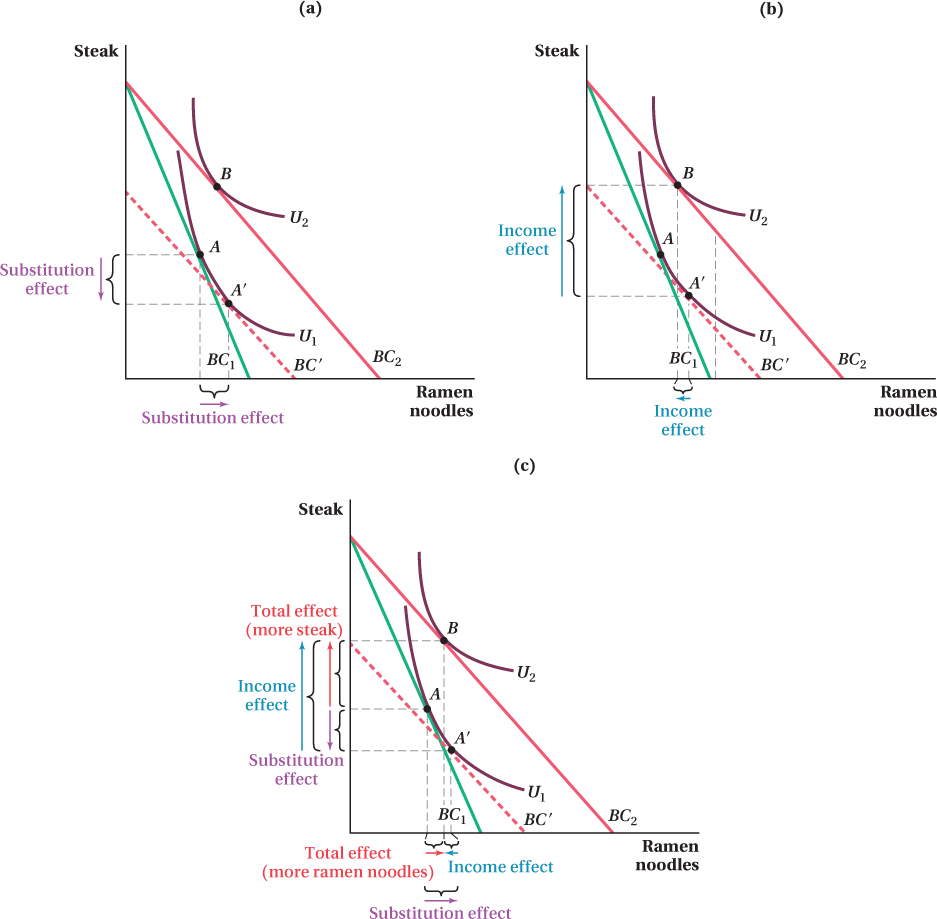 Figure 5.14: Figure 5.13 Substitution and Income Effects for an Inferior GoodFigure 5.14: (a) BC′ is the budget constraint parallel to BC2, the budget constraint after the price change, and tangent to U1, the consumer’s utility before the price change. The point of tangency between BC′ and U1, consumption bundle A′, is the bundle the consumer would purchase if relative prices changed but her purchasing power did not. The change from bundle A to bundle A′ is the substitution effect. As before, Judi chooses to purchase more of the good that has become relatively cheaper (ramen) and less of the other good (steak).Figure 5.14: (b) The change in the quantity of goods consumed from bundle A′ to B represents the income effect. Because ramen is an inferior good, the income effect leads Judi to decrease her consumption of ramen noodles, while her consumption of steak still increases.Figure 5.14: (c) The change in the quantity of goods consumed from bundle A to B represents the total effect. Since the substitution effect increases the quantity demanded by more than the income effect decreases it, Judi consumes more ramen noodles in the new optimal bundle B than in the original optimal bundle A.
The quantity shifts between bundle A′ and bundle B, shown in panel b of Figure 5.13, are due to the income effect. As before, this is the change in quantities consumed due to the shift in the budget lines from BC′ to BC2: Judi’s increase in buying power while holding relative prices constant. Notice that now the income effect here reduces the quantity of ramen noodles consumed, even though the drop in their price makes Judi richer by expanding the set of bundles she can consume. This just means ramen is an inferior good over this income range; an increase in income makes Judi want less of it.
The fact that a price drop leads to a reduction in the quantity consumed due to the income effect does not mean that the demand curve for ramen noodles slopes up because the substitution effect increases the quantity demanded by more than the income effect decreases it. Thus, the quantity of ramen noodles demanded still rises when their price falls even though ramen noodles are an inferior good. We see this outcome in panel c of Figure 5.13 because the total effect on the quantity of ramen noodles is still positive: The optimal bundle after ramen noodles become cheaper (bundle B) has a higher quantity of ramen than the optimal bundle before their price fell (bundle A). As a result, the demand curve for ramen slopes down. This is generally the case for inferior goods in the economy—
178
179
If the income effect is large enough, however, it is possible that a reduction in the price of an inferior good could actually lead to a net decrease in its consumption. A good that exhibits this trait is called a Giffen good.
Giffen Goods
Giffen good
A good for which price and quantity demanded are positively related.
Giffen goods are goods for which a fall in price leads the consumer to want less of the good. (They are named after British economist and statistician Sir Robert Giffen.) That is, an inverse relationship does not exist between price and quantity demanded and the demand curves of Giffen goods slope up! The more expensive a Giffen good is, the higher the quantity demanded. This happens because, for Giffen goods, the substitution effect of a price drop, which acts to increase the quantity a consumer demands of the good, is smaller than the reduction in the desired quantity caused by the income effect. Note that this means Giffen goods must be inferior goods.
Figure 5.14 gives a graphical example. The two goods are potatoes and meat, and potatoes are the Giffen good. The utility-
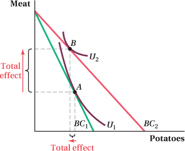
Giffen goods are extremely rare because they need to have limited substitutability with other goods (small substitution effects with highly curved indifference curves) while also having a large income effect. Large income effects generally occur when a good accounts for a large fraction of a consumer’s budget. If the price of the good falls because the consumer is already spending most of her income on it, she’s likely to feel a larger bump in effective buying power than if the good were only a small share of her budget. Finding goods that are a huge share of the budget but do not have many substitutes is really unusual.
180
Application: Someone Actually Found a Giffen Good!
While Giffen goods are theoretically possible, like Bigfoot, they seem extremely rare in practice and are often disproven on further examination. An often cited example of a Giffen good is the potato in Ireland during the Irish famine of the mid-
For one thing, if potatoes were a Giffen good for individual households, then the total market demand curve for potatoes in Ireland should have also sloped up (quantity demanded would have increased as price increased). (We will learn about how individuals’ demand curves add up to total market demand later in this chapter.) But that would mean that the huge drop in supply due to the blight—
However, a recent policy experiment with extremely poor households in rural areas of China’s Hunan province by Robert Jensen and Nolan Miller has produced what could be the most convincing documentation of a Giffen good to date.6 Jensen and Miller subsidized the purchases of rice to a randomly selected set of such households, effectively lowering the price of rice that they faced. They then compared the change in rice consumption in the subsidized households to rice consumption in unsubsidized households of similar incomes and sizes.
Jensen and Miller found that the subsidy, even though it made rice cheaper, actually caused the households’ rice consumption to fall. Rice was a Giffen good for these households. (Jensen and Miller conducted a similar experiment subsidizing wheat purchases in Gansu province and also found evidence that wheat was a Giffen good for some families, though the effect was weaker.) Rice purchases took up so much of these households’ incomes that the subsidy greatly increased the households’ effective buying power. The resulting income effect made them want to consume less rice in place of other foods for the sake of dietary variety. This income effect was large enough to outweigh the substitution effect. To oversimplify things a little, the households were initially buying enough rice to meet their caloric needs and spending their (nonexistent) leftover income on foods that added variety. When they could meet their caloric needs more cheaply, they used the now freed-
Interestingly, Jensen and Miller also found that while rice was a Giffen good for very poor households, it was not a Giffen good for the very poorest of the poor. Those extremely impoverished households basically ate only rice before the subsidy, and not really enough to meet their basic caloric needs at that. When rice became cheaper, they bought more in order to meet some basic level of healthy subsistence. Essentially, even the subsidy didn’t raise their income enough to allow them to buy any other foods besides rice. 
181
make the grade
Simple rules to remember about income and substitution effects
It is easy to get tripped up when you’re asked to identify income and substitution effects. First, remember to always start your analysis on the indifference curve associated with the consumption bundle before the price change. If you want to know why consumption changed going from one bundle to the other, you must start with the initial bundle. Next, keep in mind the key distinctions between the two effects listed in the table below.
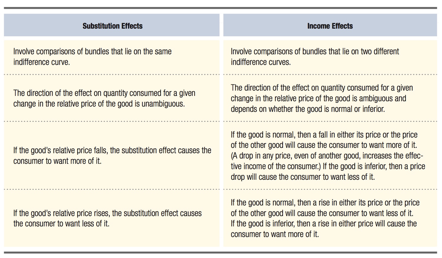
Finally, remember that the total effect of a price change (for either good) on quantity consumed depends on the relative size of the substitution and income effects. If the price of one good falls, the quantities of both goods consumed may rise, or consumption of one good may rise and consumption of the other good may decline. But the quantities consumed of both goods cannot both decline, because this would mean the consumer would not be on her budget constraint.