7.6 Economies in the Production Process
Now that we have categorized the long-
273
Economies of Scale
We talked about returns to scale in Chapter 6. Remember that a production technology has increasing returns to scale if doubling all inputs leads to more than a doubling of output. If doubling all inputs exactly doubles output, its returns to scale are constant. If output less than doubles, there are decreasing returns to scale.
economies of scale
Total cost rises at a slower rate than output rises.
diseconomies of scale
Total cost rises at a faster rate than output rises.
constant economies of scale
Total cost rises at the same rate as output rises.
Economies of scale are the cost-
Because economies of scale imply that total cost increases less than proportionately with output, they also imply that long-
Putting together these relationships, we can see what the typical U-
At the very bottom of the average total cost curve where it is flat, average cost does not change, total cost rises proportionally with output, and marginal cost equals ATC. Here, therefore, average total cost increases at the same rate that output increases, and there are constant economies of scale.
At higher output levels (the right upward-
Economies of Scale versus Returns to Scale
Economies of scale and returns to scale are not the same thing. They are related—
Because a firm can only reduce its cost more if it is able to change its input ratios when output changes, it can have economies of scale if it has constant or even decreasing returns to scale. That is, even though the firm might have a production function in which doubling inputs would exactly double output, it might be able to double output without doubling its total cost by changing the proportion in which it uses inputs. Therefore, increasing returns to scale imply economies of scale, but not necessarily the reverse.3
274
 See the problem worked out using calculus
figure it out 7.5
For interactive, step-
Suppose that the long-
Solution:
If we can find the output that minimizes long-
Minimum average cost occurs when LMC = LATC. But, we need to determine LATC before we begin. Long-
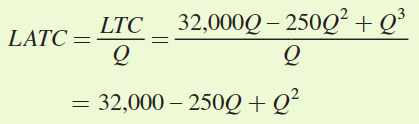
Now, we need to set LATC = LMC to find the quantity that minimizes LATC:
LATC = LMC
32,000 – 250Q + Q2 = 32,000 – 500Q + 3Q2
250Q = 2Q2
250 = 2Q
Q = 125
Long-
Application: Economies of Scale in Retail: Goodbye, Mom and Pop?
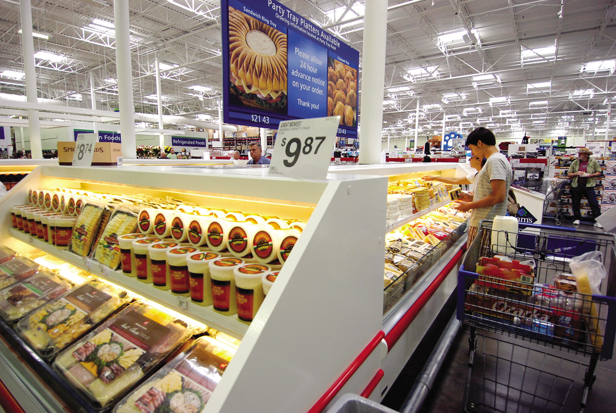
Looking at the sizes of businesses in an industry can often tell us about economies of scale in that market. Consider retailing as an example. Many folks have a sense that stores are bigger than they used to be. People once headed to the corner grocery store for a loaf of bread or a jug of milk. Now they go to the supercenter or, in some places, the hypermarket, where they can choose from a hundred kinds of bread and dozens of types of milk. Sporting goods stores were formerly the size of a couple of classrooms. Now some could hold several school buildings. And hardware stores—

The data bear out these observations. The retail sector in the U.S. has seen a move to larger stores over the past couple of decades. According to the Census of Retail Trade, there were fewer retail stores in the country in 2012 than there were 20 years earlier, despite two decades of economic and population growth. The decline is not because people are buying everything online—
Something seems to have shifted scale economies in retailing to make larger stores more efficient. One important factor is the spread of “big box” and warehouse store formats. Retailers have figured out how to stock and operate these behemoths efficiently through advances in computerized ordering, inventory, and checkout. These factors and the growing value of offering large varieties of products have created economies of scale that have encouraged the move toward larger stores. As a result, stores that are 120,000 square feet (12,000 square meters, larger than two football fields) are now common, whereas they were once unheard of. Giant stores holding massive quantities and varieties of products have replaced many of the smaller, independent “mom-
economies of scope
The simultaneous production of multiple products at a lower cost than if a firm made each product separately. 
275
Economies of Scope
Many firms make more than one product. McDonald’s sells Big Macs, Quarter Pounders, Egg McMuffins, and french fries. Just as economies of scale indicate how firms’ costs vary with the quantity they produce, economies of scope indicate how firms’ costs change when they make more than one product. Economies of scope exist when a producer can simultaneously make multiple products at a lower cost than if it made each product separately and then added up the costs.
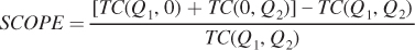
To be more explicit, let a firm’s cost of simultaneously producing Q1 units of Good 1 and Q2 units of Good 2 be equal to TC(Q1, Q2). If the firm produces Q1 units of Good 1 and nothing of Good 2, its cost is TC(Q1, 0). Similarly, if the firm produces Q2 units of Good 2 and none of Good 1, its cost is TC(0, Q2). Under these definitions, the firm is considered to have economies of scope if TC(Q1, Q2) < TC(Q1, 0) + TC(0, Q2). In other words, producing Q1 and Q2 together is cheaper than making each separately.
We can go beyond just knowing whether or not economies of scope exist, and actually quantify them in a way that allows us to compare scope economies across companies. We call this measure SCOPE, and it’s the difference between the total costs of single-
diseconomies of scope
The simultaneous production of multiple products at a higher cost than if a firm made each product separately.
If SCOPE > 0, the total cost of producing Goods 1 and 2 jointly is less than making the goods separately, so there are economies of scope. The greater SCOPE is, the larger are the firm’s cost savings from making multiple products. If SCOPE = 0, the costs are equivalent, and economies of scope are zero. And if SCOPE < 0, then it’s actually cheaper to produce Q1 and Q2 separately. In other words, there are diseconomies of scope.
276
There are two important things to remember about economies of scope. First, they are defined for a particular level of output of each good. Economies of scope might exist at one set of output levels—
Why Economies of Scope Arise
There are many possible sources of scope economies. They depend on the flexibility of inputs and the inherent nature of the products.
A common source of economies of scope is when different parts of a common input can be applied to the production of the firm’s different products. Take a cereal company that makes two cereals, Bran Bricks and Flaky Wheat. The firm needs wheat to produce either cereal. For Bran Bricks, it needs mostly the bran, the fibrous outer covering of the wheat kernel, but for Flaky Wheat, the firm needs the rest of the kernel. Therefore, there are natural cost savings from producing both cereals together.
In oil refining, the inherent chemical properties of crude oil guarantee economies of scope. Crude oil is a collection of a number of very different hydrocarbon molecules; refining is the process of separating these molecules into useful products. It is physically impossible for a refining company to produce only gasoline (or kerosene, diesel, lubricants, or whatever petroleum product might be fetching the highest price at the time). While refiners have some limited ability to change the mix of products they can pull out of each barrel of crude oil, this comes at a loss of scope economies. That’s why refineries always produce a number of petroleum compounds simultaneously.
The common input that creates scope economies does not have to be raw materials. For example, Google employees might be more productive using their knowledge about information collection and dissemination to produce multiple products (e.g., Google Earth, Google Docs, and YouTube) than to produce just the main search engine.