9.3 Profit Maximization for a Firm with Market Power
Now that we know how to compute marginal revenue, we can figure out the profit-
Many people’s first thought is that a firm with market power should sell until the marginal revenue falls to zero and then stop. After all, any more production after that would reduce revenues and wouldn’t be profitable. That idea would be correct if there was no cost of production. With production costs, however, it’s not quite right. A firm with market power should pay attention to its marginal revenue, but one more piece of the puzzle is necessary to figure out the profit-
How to Maximize Profit
In Chapter 8, we discussed the two basic elements of firm profit—
The same underlying logic works for firms with market power except that marginal revenue no longer equals price. To maximize its profit, a firm should choose its quantity where its marginal revenue equals its marginal cost:
MR = MC
If marginal revenue is above marginal cost, a firm can produce more and earn more revenue than the extra cost of production, and increase its profit. If marginal revenue is below marginal cost, a firm can reduce its output, lose less revenue than it saves in cost, and again raise its profit. Only when these two marginal values are equal does changing output not increase profit.
345
Thus, we see that the monopolist and the perfectly competitive firm do exactly the same thing. They both produce at the level where MR = MC. But because marginal revenue isn’t the same as the sales price for a firm with market power, it behaves differently than a perfectly competitive firm.
Setting MR = MC gives us the quantity, Q*, that maximizes the firm’s profit, and from that we figure out the profit-
For a firm with market power, we can think of the firm choosing a profit-
An important factor to remember is that even though firms with market power have an ability to set the price for their output, they cannot profitably charge whatever price they want to. A firm with market power can keep raising its price (or equivalently, keep cutting its output), but if the firm raises the price by too much, its customers will stop buying—
For example, in 2010 the iPad dominated the tablet market and Apple clearly had market power as a result. But Apple could not charge whatever price it wanted. Suppose Apple had charged $20,000 for each iPad. Just about everyone would have stopped buying it, even if it was the only tablet computer on earth. The vast majority of people would simply not find it worth having an iPad at that price. A monopolist doesn’t lose business to direct competitors by raising the price for its product. (A monopolist has no direct competitors.) Instead, it loses business by driving its customers out of the market. A firm is limited by the demand for its product. Because the demand curve is downward-
Profit Maximization with Market Power: A Graphical Approach
We can apply the exact logic of the previous analysis to graphically derive the profit-
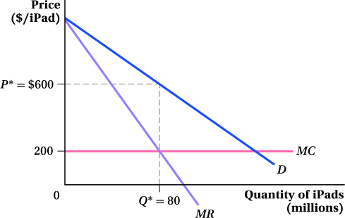
Step 1:Derive the marginal revenue curve from the demand curve. For a linear demand curve, this will be another straight line with the same vertical intercept that is twice as steep. In Figure 9.3, the marginal revenue curve is shown as MR.

Step 2:Find the output quantity at which marginal revenue equals marginal cost. This is the firm’s profit-
Step 3:Determine the profit-
346
That’s all there is to it. Once we have the firm’s MR curve, we can use the profit-
Profit Maximization with Market Power: A Mathematical Approach
We can also solve for the profit-
Suppose Apple’s marginal cost of producing iPads is constant at $200, and the demand curve for iPads (where Q is in millions and P in dollars) is Q = 200 – 0.2P. How much should Apple charge for iPads, and how many will it sell at that price? (Again, because of the equivalence of choosing price and choosing output level for firms with market power, we could ask how many iPads Apple should produce and at what price the iPads would sell, and the answer would be the same.)
We can figure this out using the same three-
Step 1: Derive the marginal revenue curve from the demand curve. Let’s start by obtaining the inverse demand curve by rearranging the demand curve so that price is a function of quantity rather than the other way around:
Q = 200 – 0.2P
0.2P = 200 – Q
P = 1,000 – 5Q
347
This is a linear inverse demand curve of the form P = a – bQ, where a = 1,000 and b = 5. Earlier we learned that MR = a – 2bQ is the marginal revenue curve for this type of demand curve.4 So for this demand curve, Apple’s marginal revenue curve is
MR = 1,000 – 2(5Q) = 1,000 – 10Q
Step 2: Find the output quantity at which marginal revenue equals marginal cost. Apple’s marginal cost is constant at $200. Therefore, we just set the marginal revenue curve equal to this value and solve for Q:
MR = MC
1,000 – 10Q = 200
800 = 10Q
Q* = 80
So, Apple’s profit-
Step 3:Determine the profit-
P* = 1,000 – 5Q*
= 1,000 – 5(80)
= 1,000 – 400 = 600
Given this demand curve and a constant marginal cost of $200 per iPad, then, Apple can maximize its profits by charging $600 per unit. It will sell 80 million iPads at this price. Notice that this price is well above Apple’s marginal cost of $200, the price Apple would be charging in a perfectly competitive market. That’s why firms like to have market power. The idea is simple: Reduce output. Raise prices. Make money.
figure it out 9.2
Babe’s Bats (BB) sells baseball bats for children around the world. The firm faces a demand curve of Q = 10 – 0.4P, where Q is measured in thousands of bats and P is dollars per bat. BB has a marginal cost curve that is equal to MC = 5Q.
Solve for BB’s profit-
maximizing level of output. Show the firm’s profit- maximization decision graphically. What price will BB charge to maximize its profit?
Solution:
To solve this problem, we should follow the three-
step procedure outlined in the text. First, we need to derive the marginal revenue curve for BB bats. Because the firm faces a linear demand curve, the easiest way to obtain the marginal revenue curve is to start by solving for the firm’s inverse demand curve: Q = 10 – 0.4P
0.4P = 10 – Q
P = 25 – 2.5Q
For this inverse demand curve, a = 25 and b = 2.5. Therefore, since MR = a – 2bQ, we know that BB’s MR curve will be
MR = 25 – 2(2.5Q) = 25 – 5Q

To solve for the profit-
maximizing level of output, we can follow the profit- maximization rule MR = MC : MR = MC
25 – 5Q = 5Q
10Q = 25
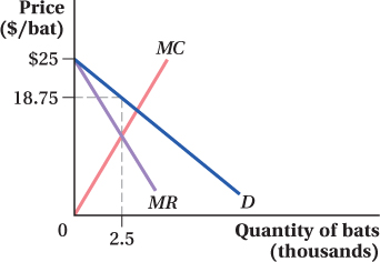
Q* = 2.5
Therefore, BB should produce 2,500 bats. This profit-
maximization decision is shown in the figure to the left. Profit is maximized at the output level at which the marginal revenue and marginal cost curves intersect. To find BB’s optimal price, we plug its profit-
maximizing level of output (Q* = 2.5) into its inverse demand curve: P* = 25 – 2.5Q*
= 25 – 2.5(2.5)
= 25 – 6.25 = 18.75
BB should charge a price of $18.75 per bat. This is also demonstrated on the figure by following Q* = 2.5 up to the demand curve and over to the vertical axis.
348
A Markup Formula for Companies with Market Power: The Lerner Index
We can take the logic we’ve just learned even further to come up with a rule-
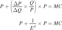
Start with the definition of MR from above:

We know that the firm maximizes its profits by setting MR = MC, so plug that in:

Now use a math trick and multiply the second term on the left side of the equation by P/P. This doesn’t change the value of the equation, because multiplying by P/P is just another way of multiplying by 1. This changes our expression to

If the section in parentheses looks familiar to you, it’s because it is the inverse of the elasticity of demand. Remember that in Chapter 2 we defined the price elasticity of demand ED as  . The inverse of this value is
  Substituting the inverse elasticity into the profit-

349
A final bit of rearranging yields

markup
The percentage of the firm’s price that is greater than its marginal cost.
The left-
If we stop to think about these implications for a minute, they make perfect sense. When demand is quite inelastic, consumers’ purchases of the firm’s product are not sensitive to changes in price. This makes it easier for the firm to increase its profit by raising its price—
Lerner index
A measure of a firm’s markup, or its level of market power.
The measure of the markup given by the equation above has a special name: the Lerner index (after Abba Lerner, the economist who proposed it in 1934). As we just discussed, assuming the firm is trying to maximize its profit, the Lerner index tells us something about the nature of the demand curve facing the firm. When the index is high (i.e., when the markup accounts for a large fraction of the price), the demand for the firm’s product is relatively inelastic. When the index is low, the firm faces relatively elastic demand. Because the ability to price above marginal cost is the definition of market power, the Lerner index is a measure of market power. The higher it is, the greater the firm’s ability to price above its marginal cost.
The extreme case of perfectly elastic demand is interesting to study in terms of its implications for the Lerner index. When demand is perfectly elastic—
Another interesting case occurs when Ed falls between 0 and –1—
350
The Lerner index can range anywhere from 0 (perfect competition) to just under 1 (barely elastic—
Measuring the Lerner Index Firms with market power know their profit-
Technologies that allow firms to change prices more frequently, and even offer different prices simultaneously to different consumers, have made firms’ processes of feeling out their demand curves easier. This can lead to negative publicity, however. For example, Amazon got into a bit of trouble early in its history for conducting what it called a “pricing experiment” on its customers. Amazon was experimentally offering different prices to different customers for the same products, in an effort to measure the elasticity of demand by seeing how consumers’ purchases responded to price changes. A customer sued when he discovered that when he removed the Amazon cookie from his computer, the price of the product he was shopping for dropped significantly. In the uproar that followed, people assumed that Amazon was price-
Application: Market Power versus Market Share

Market power involves more than the size of a particular firm. For example, consider Dr. Brown’s, a manufacturer of specialty sodas in the United States that produces a celery-
How can that be? The key factor to consider is the price elasticity of demand for the two products. Coca-
If we use these two elasticities to measure the Lerner index for each product, we indeed see that Cel-

Therefore, Cel-
351
The Supply Relationship for a Firm with Market Power
We now know how to figure out the profit-
That sounds a lot like a supply curve—
This strict relationship between costs and price isn’t true for a firm with market power. Its optimal output level depends on not only the marginal cost curve, but also the firm’s marginal revenue curve (which is related to the demand curve). Put another way, a supply curve gives a one-
 See the problem worked out using calculus