10.1 10.1 Simple Linear Regression
When you complete this section, you will be able to:
• Describe the simple linear regression model in terms of a population regression line and the distribution of deviations of the response variable y from this line.
• Use linear regression output from statistical software to find the least-
squares regression line and estimated model standard deviation.• Distinguish the model deviations ϵi from the residuals ei that are obtained from a least-
squares fit to a data set. • Use plots to visually check the assumptions of the simple linear regression model.
• Construct and interpret a level C confidence interval for the population intercept and for the population slope.
• Perform a level α significance test for the population intercept and for the population slope.
• Construct and interpret a level C confidence interval for a mean response and a level C prediction interval for a future observation when x = x*.
Statistical model for linear regression
Simple linear regression studies the relationship between a response variable y and a single explanatory variable x. We expect that different values of x will produce different mean responses for y. We encountered a similar but simpler situation in Chapter 7 when we discussed methods for comparing two population means. Figure 10.1 illustrates the statistical model for a comparison of blood pressure change in two groups of experimental subjects. Group 2 subjects were provided extra servings of fruits and vegetables in a calorie-
• The mean change in blood pressure may be different in the two populations. These means are labeled μ1 and μ2 in Figure 10.1.
Page 557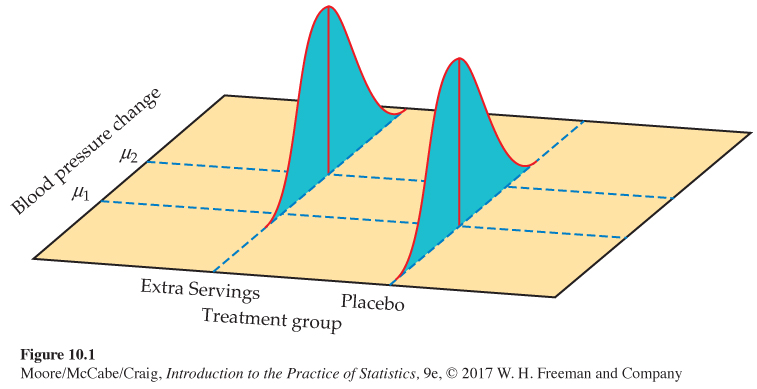 Figure 10.1: FIGURE 10.1 The statistical model for comparing responses to two treatments; the mean response varies with the treatment.
• Individual changes vary within each population according to a Normal distribution. The two Normal curves in Figure 10.1 describe these responses. These Normal distributions have the same spread, indicating that the population standard deviations are equal.
In linear regression, the explanatory variable x is quantitative and can have many different values. Imagine, for example, giving a different number of servings of fruits and vegetables x to different groups of college students. We can think of the values of x as defining different subpopulationssubpopulations, one for each possible value of x. Each subpopulation consists of all individuals in the college student population having the same value of x. If we gave x = 5 servings to some students, x = 7 servings to some others, x = 9 servings to some others, and x = 11 servings to the rest, these four groups of students would be considered samples from the corresponding four subpopulations.
The statistical model for simple linear regression assumes that for each value of x, the observed values of the response variable y are Normally distributed with a mean that depends on x. We use μy to represent these means. In general, the means μy can change as x changes according to any sort of pattern. In simple linear regressionsimple linear regression, the means all lie on a line when plotted against x. To summarize, this model also has two important parts:
• The mean blood pressure change is different for the different subpopulations of x. The means all lie on a straight line. That is, μy=β0+β1x.
• Individual blood pressure responses y with the same servings x vary according to a Normal distribution. This variation, measured by the standard deviation σ, is the same for all values of x.
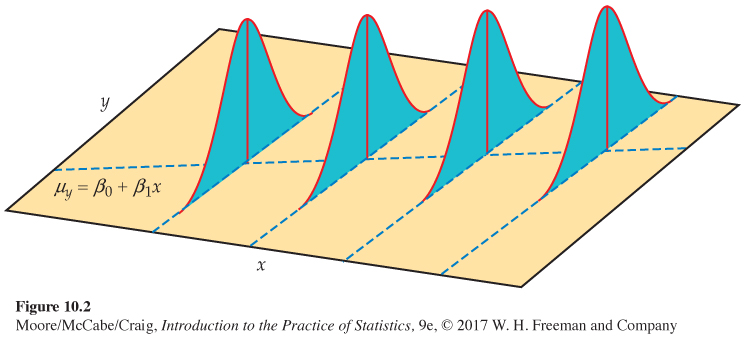
The simple linear regression model is pictured in Figure 10.2. The line describes how the mean response μy changes with x. This is the population regression linepopulation regression line. The four Normal curves show how the response y will vary for four different values of the explanatory variable x. Each curve is centered at its mean response μy. All four curves have the same spread, measured by their common standard deviation σ.
Preliminary data analysis and inference considerations
The data for a linear regression are observed values of y and x. The model takes each x to be a known quantity, like the number of servings of fruits and vegetables. The response y for a given x is assumed to be a Normal random variable. The linear regression model describes the mean and standard deviation of this random variable.
We use the following example to explain the fundamentals of simple linear regression. Because regression calculations in practice are done by statistical software, we rely on computer output for the arithmetic. In Section 10.2, we give an example that illustrates how to do the work with a calculator or spreadsheet.
EXAMPLE 10.1
Relationship between BMI and physical activity. Decrease in physical activity is considered to be a major contributor to the increase in prevalence of overweight and obesity in the general adult population. Because the prevalence of physical inactivity among college students is similar to that of the adult population, researchers have tried to understand college students’ physical activity perceptions and behaviors.

In several studies, researchers have looked at the relationship between physical activity (PA) and body mass index (BMI).1 For this study, each participant wore a FitBit FlexTM for a week, and the average number of steps taken per day (in thousands) was recorded. Various body composition variables, including BMI in kilograms per square meter, kg/m2, were also measured. We consider a sample of 100 female undergraduates.
![]()
Before starting our analysis, it is appropriate to consider the extent to which the results can reasonably be generalized. In the original study, undergraduate volunteers were obtained at a large southeastern public university through classroom announcements and campus flyers. The potential for bias should always be considered when obtaining volunteers. In this case, the participants were screened, and those with severe health issues, as well as varsity athletes, were excluded. As a result, the researchers considered these volunteers as a simple random sample (SRS) from the population of undergraduates at this university. However, they acknowledged the risks of generalizing further, stating that similar investigations at universities of different sizes and in other climates of the United States are needed.
simple random sample, p. 191
![]()
Another issue to consider in this example is the fact that the explanatory variable is not exactly known but, instead, estimated using a FitBit Flex worn over a one-
EXAMPLE 10.2
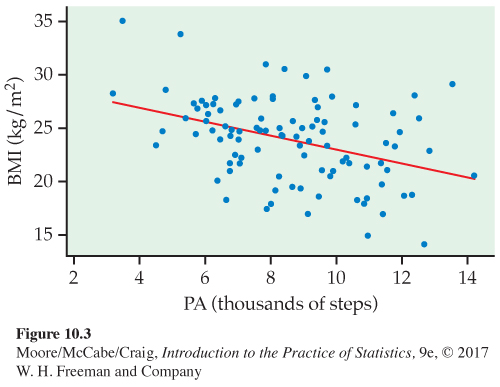
Graphical display of BMI and physical activity. We start our analysis with a scatterplot of the data. Figure 10.3 is a plot of BMI versus physical activity for our sample of 100 participants. We use the variable names BMI and PA. The least-
scatterplot, p. 86
![]()
Always start with a graphical display of the data. There is no point in fitting a linear model if the relationship is not approximately linear. A graphical display can also be used to assess the direction and strength of the relationship and to identify outliers and influential observations.
outliers and influential observations, p. 128
In this example, subpopulations are defined by the explanatory variable, physical activity. The considerable amount of scatter about the least-
The statistical model for linear regression assumes that these BMI values are Normally distributed with a mean μy that depends upon x in a linear way. Specifically,
μy = β0 + β1x
This was displayed in Figure 10.2 with the line and the four Normal curves. The line is the population regression line, which gives the average BMI for all values of x. The Normal curves provide a description of the variation of BMI about these means. The following equation expresses this idea:
DATA = FIT + RESIDUAL
The FIT part of the model consists of the subpopulation means, given by the expression β0 + β1x. The RESIDUAL part represents deviations of the data from the line of population means. We assume that these deviations are Normally distributed with mean 0 and standard deviation σ.
We use ϵ (the lowercase Greek letter epsilon) to stand for the RESIDUAL part of the statistical model. A response y is the sum of its mean and a chance deviation ϵ from the mean. These model deviations ϵ represent “noise,’’ that is, variation in y due to other causes that prevent the observed (x, y)-values from forming a perfectly straight line on the scatterplot.
SIMPLE LINEAR REGRESSION MODEL
Given n observations of the explanatory variable x and the response variable y,
(x1, y1), (x2, y2), … (xn, yn)
the statistical model for simple linear regression states that the observed response yi when the explanatory variable takes the value xi is
yi=β0+β1xi+ϵi
Here, β0 + β1xi is the mean response when x = xi. The deviations ϵi are assumed to be independent and Normally distributed with mean 0 and standard deviation σ.
The parameters of the model are β0, β1, and σ.
USE YOUR KNOWLEDGE
Question 10.1
10.1 Understanding a linear regression model. Consider a linear regression model for the decrease in blood pressure (mmHg) over a four-
(a) What is the slope of the population regression line?
(b) Explain clearly what this slope says about the change in the mean of y for a change in x.
(c) What is the subpopulation mean when x = 7 servings per day?
(d) The decrease in blood pressure y will vary about this subpopulation mean. What is the distribution of y for this subpopulation?
(e) Using the 68–
95– 99.7 rule (page 57), between what two values would approximately 95% of the observed responses, y, fall when x = 7?
10.1 (a) 0.8. (b) For each serving of fruits and vegetables in a calorie-controlled diet, the expected average decrease in blood pressure goes up by 0.8. (c) 8.4. (d) N(8.4, 3.2). (e) (2.0, 14.8).
Estimating the regression parameters
The method of least squares presented in Chapter 2 fits a line to summarize a relationship between the observed values of an explanatory variable and a response variable. Now we want to use the least-
ˆy=b0+b1x
estimate the slope β1 and the intercept β0 of the population regression line.
least-
![]()
This inference should only be done when the statistical model assumptions just presented are reasonably met. Model checks are needed and some judgment is required. Because additional methods to check model assumptions rely on first fitting the model to the data, let’s briefly review the methods of Chapter 2 concerning least-
Using the formulas from Chapter 2 (page 112), the slope of the least-
b1=rsysx
and the intercept is
b0=ˉy−b1ˉx
Here, r is the correlation between y and x, sy is the standard deviation of y, and sx is the standard deviation of x. Notice that if the slope is 0, so is the correlation, and vice versa. We discuss this relationship more later in the chapter.
correlation, p. 101
The predicted value of y for a given value x* of x is the point on the least-
ei=observed response− predicted response=yi−ˆy=yi−b0−b1xi
The residuals ei correspond to the linear regression model deviations ϵi. The ei sum to 0, and the ϵi come from a population with mean 0. Because we do not observe the ϵi, we use the residuals to check the model assumptions of the ϵi.
Recall that the least-
The remaining parameter to be estimated is σ, which measures the variation of y about the population regression line. Because this parameter is the standard deviation of the model deviations, it should come as no surprise that we use the residuals to estimate it. As usual, we work first with the variance and take the square root to obtain the standard deviation.
For simple linear regression, the estimate of σ2 is the average squared residual
sample variance, p. 38
s2=∑e2in−2=∑(yi−ˆyi)2n−2
We average by dividing the sum by n − 2 in order to make s2 an unbiased estimate of σ2 (the sample variance of n observations uses the divisor n − 1 for this same reason). The quantity n − 2 is called the degrees of freedom for s2. The estimate of the model standard deviation σmodel standard deviation σ is given by
s=√s2
We now use statistical software to calculate the regression for predicting BMI from physical activity for Example 10.1. In entering the data, we chose the names PA for the explanatory variable and BMI for the response. It is good practice to use names, rather than just x and y, to remind yourself which variables the output describes.
EXAMPLE 10.3
Statistical software output for BMI and physical activity. Figure 10.4 gives the outputs from three commonly used statistical software packages and Excel. Other software will give similar information. The SPSS output reports estimates of our three parameters as b0 = 29.578, b1 = −0.655, and s = 3.6549. Be sure that you can find these values in this output and the corresponding values in the other outputs.
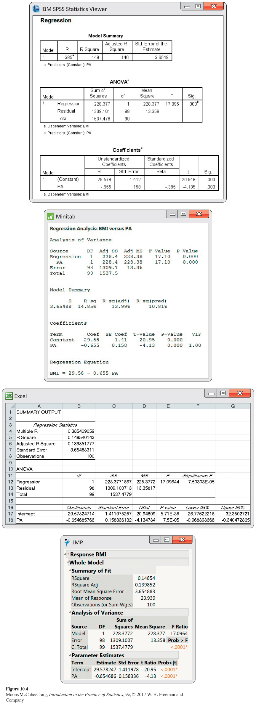
The least-
^BMI=29.578−0.655PA
with an estimated model standard deviation of s = 3.655. It says that for each increase of 1000 steps per day, we expect the average BMI to be 0.655 smaller. The large estimated model standard deviation, however, suggests there is a lot of variability about these means.
![]()
Note that the number of digits provided varies with the software used, and we have rounded the values to three decimal places. It is important to avoid cluttering up your report of the results of a statistical analysis with many digits that are not relevant. Software often reports many more digits than are meaningful or useful.
The outputs contain other information that we will ignore for now. Computer outputs often give more information than we want or need. This is done to reduce user frustration when a software package does not print out the particular statistics wanted for an analysis. The experienced user of statistical software learns to ignore the parts of the output that are not needed for the current analysis.
EXAMPLE 10.4
Predicted values and residuals for BMI. We can use the least-
29.578 − 0.655(8) = 24.338
If her actual BMI is 25.655, then the residual would be
y−ˆy=25.655−24.338=1.317
Because the means μy lie on the line μy = β0 + β1x, they are all determined by β0 and β1. Thus, once we have estimates of β0 and β1, the linear relationship determines the estimates of μy for all values of x. Linear regression allows us to do inference not only for subpopulations for which we have data but also for those corresponding to x’s not present in the data. These x-values can be both within and outside the range of observed x’s. However, extreme caution must be taken when performing inference for an x-value outside the range of the observed x’s because there is no assurance that the same linear relationship between μy and x holds.
extrapolation, p. 110
USE YOUR KNOWLEDGE
Question 10.2
10.2 More on BMI and physical activity. Refer to Examples 10.3 (page 562) and 10.4 (page 564).
(a) What is the predicted BMI for a woman who averages 9500 steps per day?
(b) If an observed BMI at x = 9.5 were 24.3, what would be the residual?
(c) Suppose that you wanted to use the estimated population regression line to examine the predicted BMI for a woman who averages 4000, 10,000, or 16,000 steps per day. Discuss the appropriateness of using the least-
squares equation to predict BMI for each of these activity levels.
Checking model assumptions
![]()
Now that we have fitted a line, we can further check the conditions that the simple linear regression model imposes on this fit. These checks are very important to do and often overlooked. There is no point in trying to do statistical inference if the data do not, at least approximately, meet the conditions that are the foundation for the inference. Misleading or incorrect conclusions can result.
These conditions concern the population, but we can observe only our sample. Thus, in doing inference, we act as if the sample is an SRS from the population. When the data are collected through some sort of random sampling, this assumption is often easy to justify. In other settings, this assumption requires more thought, and the justification is often debatable. For example, in Example 10.1 (page 558), the sample was a collection of volunteers and the researchers argued they could be considered an SRS from the population of college students at that university.
The remaining model conditions can be checked through a visual examination of the residuals. The first condition is that there is a linear relationship in the population, and the second is that the standard deviation of the responses about the population line is the same for all values of the explanatory variable. It is common to plot the residuals both against the case number (especially if this reflects the order in which the observations were collected) and against the explanatory variable. These residual plots are preferred to scatterplots of y versus x because they better magnify patterns.
Figure 10.5 is a plot of the residuals versus physical activity with a smooth-
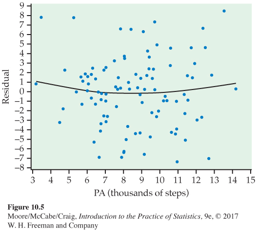
To check the assumption of a common standard deviation, we look at the spread of the residuals across the range of x. In Figure 10.5, the spread is roughly uniform across the range of PA, suggesting that this assumption is reasonable. There also do not appear to be any outliers or influential observations.
Normal quantile plot, p. 66
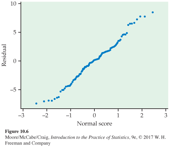
The final condition is that the response varies Normally about the population regression line. That is, the model deviations vary Normally about 0. Figure 10.6 is a Normal quantile plot of the residuals. Because the plot looks fairly straight, we are confident that we do not have a serious violation of the assumption that the model deviations are Normally distributed.
LINEAR REGRESSION MODEL CONDITIONS
To use the least-
• The sample is an SRS from the population.
• There a linear relationship between x and y.
• The standard deviation of the responses y about the population regression line is the same for all x.
• The model deviations are Normally distributed.
In summary, the data of Example 10.1 give no reason to doubt the simple linear regression model. We can comfortably proceed to inference about parameters, or functions of parameters, such as
• The slope β1 and the intercept β0 of the population regression line.
• The mean response μy for a given value of x.
• An individual future response y for a given value of x.
If these assumption checks were to raise doubts, it is best to consult an expert, as a more sophisticated regression model is likely needed. There is, however, one relatively simple remedy that may be worth investigation. This is described at the end of this section.
Confidence intervals and significance tests
Chapter 7 presented confidence intervals and significance tests for means and differences in means. In each case, inference rested on the standard errors of estimates and on t distributions. Inference in simple linear regression is similar in principle. For example, the confidence intervals have the form
estimate ± t*SEestimate
where t* is a critical point of a t distribution. The formulas for the estimate and standard error, however, are more complicated.
As a consequence of the model assumptions about the deviations ϵi, the sampling distributions of b0 and b1 are Normally distributed with means β0 and β1 and standard deviations that are multiples of σ, the model parameter that describes the variability about the true regression line. In fact, even if the ϵi are not Normally distributed, a general form of the central limit theorem tells us that the distributions of b0 and b1 will be approximately Normal.
central limit theorem, p. 298
Because we do not know σ, we use the estimated model standard deviation s, which measures the variability of the data about the least-
CONFIDENCE INTERVAL AND SIGNIFICANCE TEST FOR THE REGRESSION SLOPE
A level C confidence interval for the slope β1 is
b1±t*SEb1
In this expression, t* is the value for the t(n − 2) density curve with area C between −t* and t*.
To test the hypothesis H0: β1 = 0, compute the test statistic
t=b1SEb1
The degrees of freedom are n − 2. In terms of a random variable T having the t(n − 2) distribution, the P-value for a test of H0 against
Ha: β1 > 0 is P(T ≥ t) 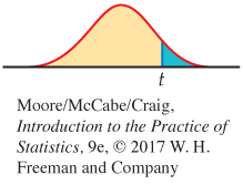
Ha: β1 < 0 is P(T ≤ t) 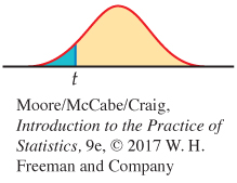
Ha: β1 ≠ 0 is 2P(T ≥ |t|) 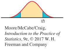
Formulas for confidence intervals and significance tests for the intercept β0 are exactly the same, replacing b1 and SEb1 by b0 and its standard error SEb0. Although computer outputs often include a test of H0: β0 = 0, this information usually has little practical value. From the equation for the population regression line, μy = β0 + β1x, we see that β0 is the mean response corresponding to x = 0. In many practical situations, this subpopulation does not exist or is not interesting.
On the other hand, the test of H0: β1 = 0 is quite useful. When we substitute β1 = 0 in the model, the x term drops out and we are left with
μy = β0
This equation says that the mean of y does not vary with x. In other words, all the y’s come from a single population with mean β0, which we would estimate by ˉy. The hypothesis H0: β1 = 0 therefore says that there is no straight-
EXAMPLE 10.5
Statistical software output, continued. The computer outputs in Figure 10.4 (pages 562–
The t statistic and P-value for the test of H0: β1 = 0 against the two-
t=b1SEb1=−0.6546960.158336=−4.13
The P-value is given as <0.0001. The other outputs in Figure 10.4 also indicate that the P-value is very small. Less than one chance in 10,000 is sufficiently small for us to decisively reject the null hypothesis.
We have found a statistically significant linear relationship between physical activity and BMI. The estimated slope is more than 4 standard deviations away from zero. Because this is highly unlikely to happen if the true slope is zero, we have strong evidence for our claim.
![]()
Note, however, that this is not the same as concluding that we have found a strong linear relationship between the response and explanatory variables in this example. We saw in Figure 10.3 that there is a lot of scatter about the regression line. A very small P-value for the significance test for a zero slope does not necessarily imply that we have found a strong relationship.
A confidence interval provides additional information about the linear relationship. For most statistical software, these intervals are optional output and must be requested. We can also construct them by hand from the default output.
EXAMPLE 10.6
Confidence interval for the slope. A confidence interval for β1 requires a critical value t* from the t(n − 2) = t(98) distribution. In Table D, there are entries for 80 and 100 degrees of freedom. The values for these rows are very similar. To be conservative, we will use the larger critical value, for 80 degrees of freedom. Find the confidence level values at the bottom of the table. In the 95% confidence column, the entry for 80 degrees of freedom is t* = 1.990.
To compute the 95% confidence interval for β1, we combine the estimate of the slope with the margin of error:
b1±t*SEb1=−0.655±(1.990)(0.158)
= −0.655 ± 0.314
The interval is (−0.969, −0.341). As expected, this is slightly wider than the interval given by software (see Excel output in Figure 10.4). We estimate that, on average, an increase of 1000 steps per day is associated with a decrease in BMI of between 0.341 and 0.969 kg/m2.
Note that the intercept in this example is not of practical interest. It estimates average BMI when the activity level is 0, a value that isn’t realistic. For this reason, we do not compute a confidence interval for β0 or discuss the significance test available in the software.
USE YOUR KNOWLEDGE
Question 10.3
10.3 Significance test for the slope. Test the null hypothesis that the slope is zero versus the two-
(a) n = 20, ˆy=28.5+1.4x, and SEb1=0.65.
(b) n = 30, ˆy=30.8+2.1x, and SEb1=1.05.
(c) n = 100, ˆy=29.3+2.1x, and SEb1=1.05.
10.3 (a) t = 2.154, df = 19, 0.04 < P-value < 0.05. (b) t = 2, df = 29, 0.05 < P-value < 0.10. (c) t = 2, df = 99, 0.04 < P-value < 0.05.
Question 10.4
10.4 95% confidence interval for the slope. For each of the settings in the previous exercise, find the 95% confidence interval for the slope and explain what the interval means.
Confidence intervals for mean response
Besides performing inference about the slope (and sometimes the intercept) in a linear regression, we may want to use the estimated regression line to make predictions about the response y at certain values of x. We may be interested in the mean response for different subpopulations or in the response of future observations at different values of x. In either case, we would want an estimate and associated margin of error.
For any specific value of x, say x*, the mean of the response y in this subpopulation is given by
μy=β0+β1x*
To estimate this mean from the sample, we substitute the estimates b0 and b1 for β0 and β1:
ˆμy=b0+b1x*
A confidence interval for μy adds to this estimate a margin of error based on the standard error SEˆμ. The formula for the standard error is given in Section 10.2.
CONFIDENCE INTERVAL FOR A MEAN RESPONSE
A level C confidence interval for the mean response μy when x takes the value x* is
ˆμy±t*SEˆμ
where t* is the value for the t(n − 2) density curve with area C between −t* and t*.
Many computer programs calculate confidence intervals for the mean response corresponding to each of the x-values in the data. Some can calculate an interval for any value x* of the explanatory variable. We will use a plot to illustrate these intervals.
EXAMPLE 10.7
Confidence intervals for the mean response. Figure 10.7 shows the upper and lower confidence limits on a graph with the data and the least-
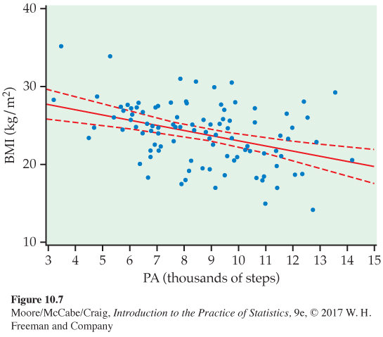
Some software will do these calculations directly if you input a value for the explanatory variable. Other software will calculate the intervals for each value of x in the data set. Creating a new data set with an additional observation with x equal to the value of interest and y missing will often work.
EXAMPLE 10.8
Confidence interval for an average of 9000 steps per day. Let’s find the confidence interval for the average BMI at x = 9.0. Our predicted BMI is
^BMI = 29.578 − 0.655PA
= 29.578 − 0.655(9.0)
= 23.7
Software tells us that the 95% confidence interval for the mean response is 23.0 to 24.4 kg/m2.
![]()
If we sampled many women who averaged 9000 steps per day, we would expect their average BMI to be between 23.0 and 24.4 kg/m2. Note that many of the observations in Figure 10.7 lie outside the confidence bands. These confidence intervals do not tell us what BMI to expect for a single observation at a particular average steps per day. We need a different kind of interval, a prediction interval, for this purpose.
Prediction intervals
In the last example, we predicted the average BMI for x* = 9000 steps per day. Suppose that we now want to predict an observation of BMI for a woman averaging 9000 steps per day. The predicted response y for an individual case with a specific value x* of the explanatory variable x is
ˆy=b0+b1x*
This is the same as the expression for ˆμy. That is, the fitted line is used both to estimate the mean response when x = x* and to predict a single future response. We use the two notations ˆμy and ˆy to remind ourselves of these two distinct uses.
This means our best guess for the BMI of this woman averaging 9000 steps per day is what we obtained using the regression equation, 23.7 kg/m2. A useful prediction, however, also needs a margin of error (or interval) to indicate its precision. The interval used to predict a future observation is called a prediction intervalprediction interval. Although the response y that is being predicted is a random variable, the interpretation of a prediction interval is similar to that for a confidence interval.
Consider doing the following many times:
• Draw a sample of n observations (xi, yi) and then one additional observation (x*, y).
• Calculate the 95% prediction interval for y when x = x* using the sample of size n.
Then, 95% of the prediction intervals will contain the value of y for the additional observation. In other words, the probability that this method produces an interval that contains the value of a future observation is 0.95.
The form of the prediction interval is very similar to that of the confidence interval for the mean response. The difference is that the standard error SEˆy used in the prediction interval includes both the variability due to the fact that the least-
PREDICTION INTERVAL FOR A FUTURE OBSERVATION
A level C prediction interval for a future observation on the response variable y from the subpopulation corresponding to x* is
ˆy±t*SEˆy
where t* is the value for the t(n − 2) density curve with area C between −t* and t*.
Again, we use a graph to illustrate the results.
EXAMPLE 10.9
Prediction intervals for BMI. Figure 10.8 shows the upper and lower prediction limits, along with the data and the least-
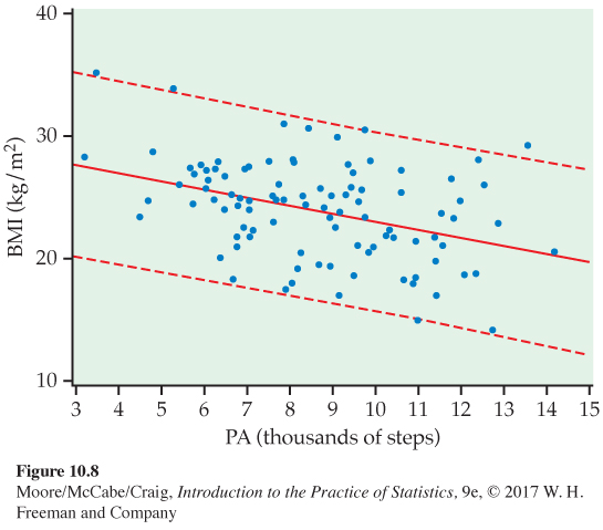
The comparison of Figure 10.7 and 10.8 reminds us that the interval for a single future observation must be larger than an interval for the mean of its subpopulation.
EXAMPLE 10.10
Prediction interval for 9000 steps per day. Let’s find the prediction interval for a future observation of BMI for a college-
![]()
Although a larger sample would better estimate the population regression line, it would not reduce the degree of scatter about the line. This means that prediction intervals for BMI, given activity level, will always be wide. This example clearly demonstrates that a very small P-value for the significance test for a zero slope does not necessarily imply that we have found a strong predictive relationship.
USE YOUR KNOWLEDGE
Question 10.5
10.5 Margin of error for the predicted mean. Refer to Figure 10.7 and Example 10.8 (page 571). What is the 95% margin of error of ˆμy when x = 9.0? Would you expect the margin of error to be larger, smaller, or the same for x = 11.0? Explain your answer.
10.5 0.7. At x = 11.0, the margin of error there will be larger.
Question 10.6
10.6 Margin of error for a predicted response. Refer to Example 10.10. What is the 95% margin of error of ˆy when x = 9.0? If you increased the sample size from n = 100 to n = 400, would you expect the 95% margin of error for the predicted response to be roughly twice a large, half as large, or the same for x = 9.0? Explain your answer.
Transforming variables
We started our analysis of Example 10.1 with a scatterplot to check whether the relationship between BMI and physical activity could be summarized with a straight line. We followed the least-
log transformation, p. 91
When there is a violation, it is best to consult an expert. However, there are times when a transformation of one or both variables will remedy the situation. In Chapter 2, we discussed the use of the log transformation to describe a curved relationship between x and y. Here is an example where the log transformation has more of an impact on other model assumptions.
EXAMPLE 10.11
The relationship between income and education for entrepreneurs. Numerous studies have shown that better-

The researchers defined entrepreneurs to be those who were self-
EXAMPLE 10.12
Graphical display of the income and education relationship. Figure 10.9 is a plot of income versus eduction for our sample of 100 entrepreneurs. We use the variable names INC and EDUC. The least-
The most striking feature of the plot is not the lack of linearity (there is some suggested curvature between y and x), but rather the distribution of income about the least-
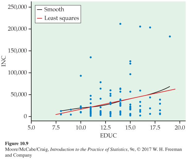
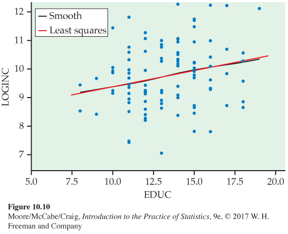
A common remedy for a strongly skewed variable is to consider transforming the variable prior to fitting the model. In this example, the researchers considered the natural logarithm of income (LOGINC).
EXAMPLE 10.13
Is this linear regression model reasonable? Figure 10.10 is a scatterplot of these transformed data with the new least-
![]()
A complete check of the residuals is still needed (see Exercise 10.11), but it appears that transforming y results in a data set that satisfies the linear regression model. Not only is the relationship more linear, but the distribution of the observations about the regression line is more Normal. This is not always the end result of a transformation. In other cases, transforming a variable may help linearity and harm the Normality and constant variance assumptions. Always check the residuals before proceeding with inference.
BEYOND THE BASICS
Nonlinear Regression
When the relationship is not linear and a transformation does not work, we often use models that allow for various types of curved relationships. These models are called nonlinear modelsnonlinear models.
The technical details are much more complicated for nonlinear models. In general, we cannot write down simple formulas for the parameter estimates; we use a computer to solve systems of equations to find the estimates. However, the basic principles are those that we have already learned. For example,
DATA = FIT + RESIDUAL
still applies. The FIT is a nonlinear (curved) function, and the residuals are assumed to be an SRS from the N(0, σ) distribution. The nonlinear function contains parameters that must be estimated from the data. Approximate standard errors for these estimates are part of the standard output provided by software. Here is an example.
EXAMPLE 10.14
Investing in one’s bone health. As we age, our bones become weaker and are more likely to break. Osteoporosis (or weak bones) is the major cause of bone fractures in older women. Various researchers have studied this problem by looking at how and when bone mass is accumulated by young women. They’ve determined that up to 90% of a person’s peak bone mass is acquired by age 18 in girls.3 This makes youth the best time to invest in stronger bones.
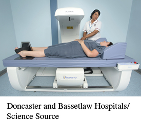
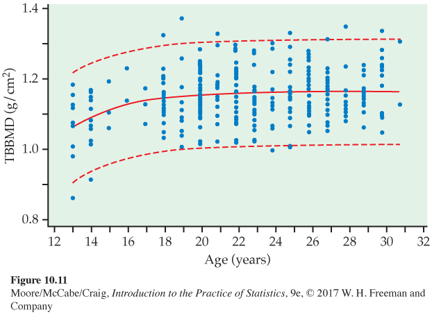
Figure 10.11 displays data for a measure of bone strength, called “total body bone mineral density’’ (TBBMD), and age for a sample of 256 young women.4 TBBMD is measured in grams per square centimeter (g/cm2), and age is recorded in years. The solid curve is the nonlinear fit, and the dashed curves are 95% prediction limits. Similar to our example of BMI and activity level, there is a large amount of scatter about the fitted curve. Although prediction intervals may be useless in this case, the researchers can draw some conclusions regarding the relationship.
The fitted nonlinear equation is
ˆy=1.162e−1.162+0.28x1+e−1.162+0.28x
In this equation, ˆy is the predicted value of TBBMD, the response variable, and x is age, the explanatory variable. A straight line would not do a very good job of summarizing the relationship between TBBMD and age. At first, TBBMD increases with age, but then it levels off as age increases. The value of the function where it is level is called “peak bone mass’’; it is a parameter in the nonlinear model. The estimate is 1.162 and the standard error is 0.008. Software gives the 95% confidence interval as (1.146, 1.178). Other calculations could be done to determine the age by which 90% of this peak bone mass is acquired.
The long-