12.1 12.1 Inference for One-Way Analysis of Variance
When you complete this section, you will be able to:
• Describe the one-
way ANOVA model and when it is used for inference.• Describe the underlying idea of the ANOVA F test in terms of the variation between population means and the variation within populations.
• Summarize what the ANOVA F test can tell you about the population means and what it cannot.
• Construct an ANOVA table with sources of variation and degrees of freedom. Compute mean squares and the F statistic when provided various sums of squares.
• Use ANOVA output to obtain the ANOVA F test results and the coefficient of determination.
• Use residual plots and sample statistics to check the assumptions of the one-
way ANOVA model.
When comparing different populations or treatments, the data are subject to sampling variability. For example, we would not expect to observe exactly the same sales data if we mailed an advertising offer to different random samples of households. We also wouldn’t expect a new group of cancer patients to provide the same set of progression-
comparing two means, p. 432
In Chapter 7, we met procedures for comparing the means of two populations. We now extend those methods to problems involving more than two populations. The statistical methodology for comparing several means is called analysis of variance, or simply ANOVAANOVA. In this and the following section, we will examine the basic ideas and assumptions that are needed for ANOVA. Although the details differ, many of the concepts are similar to those discussed in the two-
We will consider two ANOVA techniques. When there is only one way to classify the populations of interest, we use one-
In many other comparative studies, there is more than one way to classify the populations. For the tire study, the researcher may also want to consider temperature. Are there brands that do relatively better in a cooler environment? Analyzing the effect of two factors, brand and temperature, requires two-
Data for one-
One-
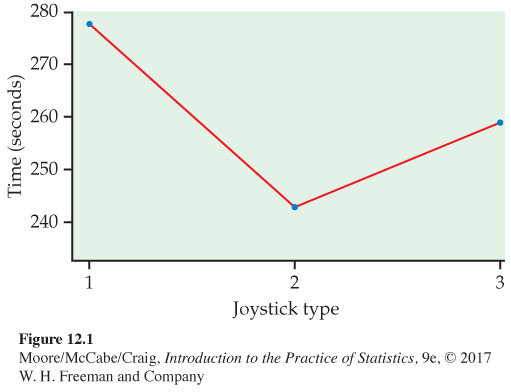
EXAMPLE 12.1

Does haptic feedback improve performance? A group of technology students is interested in whether haptic feedback (forces and vibrations applied through a joystick) is helpful in navigating a simulated game environment they created. To investigate this, they randomly assign 20 students to each of three joystick controller types and record the time it takes to complete a navigation mission. The joystick types are (1) a standard video game joystick, (2) a game joystick with force feedback, and (3) a game joystick with vibration feedback.
EXAMPLE 12.2
Average age of coffeehouse customers. How do five coffeehouses around campus differ in the demographics of their customers? Are certain coffeehouses more popular among graduate students? Do professors tend to favor one coffeehouse? A market researcher asks 50 customers of each coffeehouse to respond to a questionnaire. One variable of interest is the customer’s age.
These two examples are similar in that
• There is a single quantitative response variable measured on many units; the units are students in the first example and customers in the second.
• The goal is to compare several populations: students using different joystick types in the first example and customers of five coffeehouses in the second.
There is, however, an important difference. Example 12.1 describes an experiment in which each student is randomly assigned to a type of joystick. Example 12.2 is an observational study in which customers are selected during a particular time period and not all agree to provide data. These samples of customers are not random samples, but we will treat them as such because we believe that the selective sampling and nonresponse are ignorable sources of bias and variability. This will not always be the case. Always consider the sampling design and various sources of bias in an observational study.
![]()
In both examples, we will use ANOVA to compare the mean responses. The same ANOVA methods apply to data from randomized experiments and to data from random samples. However, it is important to keep the data-
Comparing means
The question we ask in ANOVA is “Do all groups have the same population mean?’’ We will often use the term groups for the populations to be compared in a one-
The purpose of ANOVA is to assess whether the observed differences among sample means are statistically significant. Could a variation among the three sample means this large be plausibly due to chance, or is it good evidence for a difference among the population means? This question can’t be answered from the sample means alone. Because the standard deviation of a sample mean ˉx is the population standard deviation σ divided by √n, the answer also depends upon both the variation within the groups of observations and the sizes of the samples.
standard deviation of ˉx, p. 297
Side-
Even the boxplots omit essential information, however. To assess the observed differences, we must also know how large the samples are. Nonetheless, boxplots are a good preliminary display of the data.
Although ANOVA compares means and boxplots display medians, these two measures of center will be close together for distributions that are nearly symmetric. This is something we will need to check prior to inference. If the distributions are strongly skewed, we may consider a transformation prior to displaying and analyzing the data.

The two-
Two-
t=ˉx1−ˉx2sp√1n+1n=√n2 (ˉx1−ˉx2)sp
The square of this t statistic is
t2=n2(ˉx1−ˉx2)2s2p
If we use ANOVA to compare two populations, the ANOVA F statistic is exactly equal to this t2. Thus, we learn something about how ANOVA works by looking carefully at the statistic in this form.
The numerator in the t2 statistic measures the variation betweenbetween-
The denominator measures the variation withinwithin-
Although the general form of the F statistic is more complicated, the idea is the same. To assess whether several populations all have the same mean, we compare the variation among the means of several groups with the variation within groups. Because we are comparing variation, the method is called analysis of variance.
An overview of ANOVA
ANOVA tests the null hypothesis that the population means are all equal. The alternative is that they are not all equal. This alternative could be true because all the means are different or simply because one of them differs from the rest. This is a more complex situation than comparing just two populations. If we reject the null hypothesis, we need to perform some further analysis to draw conclusions about which population means differ from which others and by how much.
The computations needed for ANOVA are more lengthy than those for the t test. For this reason, we generally use computer programs to perform the calculations. Automating the calculations frees us from the burden of arithmetic and allows us to concentrate on interpretation.
![]()
We should always start our ANOVA with a careful examination of the data using graphical and numerical summaries. Complicated computations do not guarantee a valid statistical analysis. Just as in linear regression, outliers and extreme deviations from Normality can invalidate the computed results.
EXAMPLE 12.3
Number of Facebook friends. A feature of each Facebook user’s profile is the number of Facebook “friends,’’ an indicator of the user’s social network connectedness. Among college students on Facebook, the average number of Facebook friends has been estimated to be around 650.1
Offline, having more friends is associated with higher ratings of positive attributes such as likability and trustworthiness. Is this also the case with Facebook friends?
An experiment was run to examine the relationship between the number of Facebook friends and the user’s perceived social attractiveness.2 A total of 134 undergraduate participants were randomly assigned to observe one of five Facebook profiles. Everything about the profile was the same except the number of friends, which appeared on the profile as 102, 302, 502, 702, or 902.
After viewing the profile, each participant was asked to fill out a questionnaire on the physical and social attractiveness of the profile user. Each attractiveness score is an average of several seven-
| Number of friends |
n | ˉx | s |
|---|---|---|---|
| 102 | 24 | 3.82 | 1.00 |
| 302 | 33 | 4.88 | 0.85 |
| 502 | 26 | 4.56 | 1.07 |
| 702 | 30 | 4.41 | 1.43 |
| 902 | 21 | 3.99 | 1.02 |
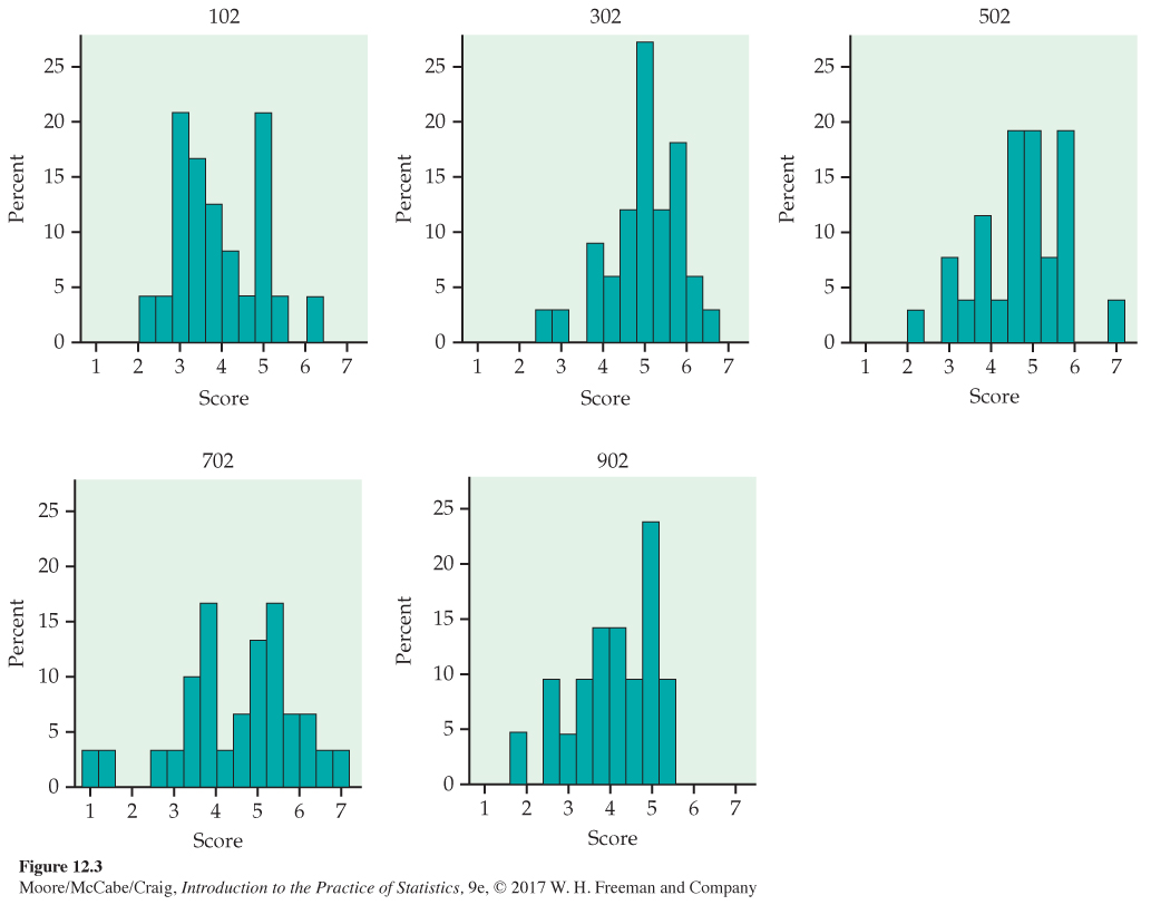
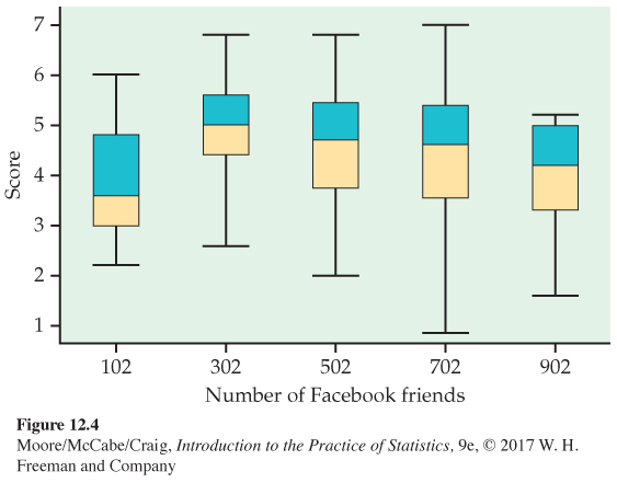
Histograms for the five groups are given in Figure 12.3. Note that the heights of the bars in the histograms are percents rather than counts. This is commonly done when the group sample sizes vary. Figure 12.4 gives side-
guidelines for two-
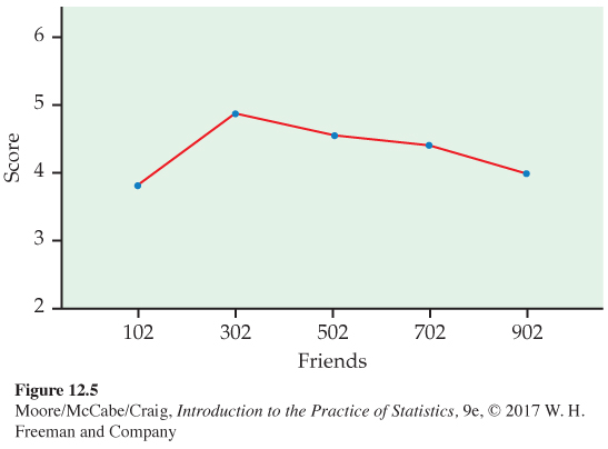
The five sample means are plotted in Figure 12.5 (page 650). They rise and then fall as the number of friends increases. This suggests that having too many Facebook friends can harm a user’s social attractiveness. However, given the variability in the data, this pattern could also just be the result of chance variation. We will use ANOVA to make this determination.
In this setting, we have an experiment in which undergraduate Facebook users were randomly assigned to view one of five Facebook profiles. Each of these profile populations has a mean, and our inference asks questions about these means. The undergraduates in this study were all from the same university. They also volunteered in exchange for course credit.
![]()
Formulating a clear definition of the populations being compared with ANOVA can be difficult. Often some expert judgment is required, and different consumers of the results may have differing opinions. Whether we can comfortably generalize our conclusions of this study to the population of undergraduates at the university or to the population of all undergraduates in the United States is open for debate. Regardless, we are more confident in generalizing our conclusions to similar populations when the results are clearly significant than when the level of significance just barely passes the standard of P = 0.05.
We first ask whether or not there is sufficient evidence in the data to conclude that the corresponding population means are not all equal. Our null hypothesis here states that the population mean score is the same for all five Facebook profiles. The alternative is that they are not all the same.
![]()
Our inspection of the data for our example suggests that the means may follow a curvilinear relationship. Rejecting the null hypothesis that the means are all the same using ANOVA is not the same as concluding that all the means are different from one another. The ANOVA null hypothesis can be false in many different ways. Additional analysis is required to distinguish among these possibilities.
![]()
When there are particular versions of the alternative hypothesis that are of interest, we use contrastscontrasts to examine them. In our example, we might want to test whether there is a curvilinear relationship between the number of friends and attractiveness score. Note that, to use contrasts, it is necessary that the questions of interest be formulated before examining the data. It is inappropriate to make up these questions after analyzing the data.
If we have no specific relations among the means in mind before looking at the data, we instead use a multiple-
USE YOUR KNOWLEDGE
Question 12.1
12.1 What’s wrong? In each of the following, identify what is wrong and then either explain why it is wrong or change the wording of the statement to make it true.
(a) ANOVA tests the null hypothesis that the sample means are all equal.
(b) A strong case for causation is best made in an observational study.
(c) You use ANOVA to compare the variances of the populations.
(d) A multiple-
comparisons procedure is used to compare a relation among means that was specified prior to looking at the data.
12.1 (a) ANOVA tests the null hypothesis that the population means are all equal. (b) Experiments are best for establishing causation. (c) ANOVA is used to compare means (and assumes that the variances are equal). (d) Multiple comparisons procedures are used when we wish to determine which means are significantly different, but we do not need specific relations in mind prior to looking at the data.
Question 12.2
12.2 What’s wrong? For each of the following, explain what is wrong and why.
(a) In rejecting the null hypothesis, one can conclude that all the means are different from one another.
(b) A one-
way ANOVA can be used only when there are two means to be compared. (c) The ANOVA F statistic will be large when the within-
group variation is much larger than the between- group variation. (d) ANOVA is insensitive to outliers and extreme departures from Normality.
The ANOVA model
When analyzing data, the following equation reminds us that we look for an overall pattern and deviations from it:
DATA = FIT + RESIDUAL
DATA = FIT + RESIDUAL, p. 560
In the regression model of Chapter 10, the FIT was the population regression line, and the RESIDUAL represented the deviations of the data from this line. We now apply this framework to describe the statistical models used in ANOVA. These models provide a convenient way to summarize the assumptions that are the foundation for our analysis. They also give us the necessary notation to describe the calculations needed.
First, recall the statistical model for a random sample of observations from a single Normal population with mean μ and standard deviation σ. If the observations are
Normal distributions, p. 56
x1, x2, . . . , xn
we can describe this model by saying that the xj are an SRS from the N(μ, σ) distribution. Another way to describe the same model is to think of the x’s varying about their population mean. To do this, write each observation xj as
xj=μ+ϵj
The ϵj are then an SRS from the N(0, σ) distribution. Because μ is unknown, the ϵ’s cannot actually be observed. This form more closely corresponds to our
DATA = FIT + RESIDUAL
way of thinking. The FIT part of the model is represented by μ. It is the systematic part of the model, like the line in a regression. The RESIDUAL part is represented by ϵj. It represents the deviations of the data from the fit and is due to random, or chance, variation.
There are two unknown parameters in this statistical model: μ and σ. We estimate μ by ˉx, the sample mean, and σ by s, the sample standard deviation. The differences ej=xj−ˉx are the residuals and correspond to the ϵj in the statistical model.
The model for one-
THE ONE-
Consider SRSs from each of I populations, with the sample from the ith population having ni observations denoted xi1, xi2, . . . , xinixi1, xi2, . . . , xini. The one-
xij=μi+ϵij
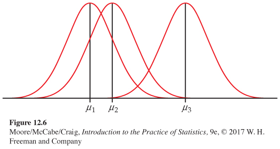
for i = 1, . . . , I and j=1, …, ni.. The ϵij are assumed to be from an N(0, σ) distribution. The parameters of the model are the population means μ1, μ2, . . . , μI and the common standard deviation σ.
Note that the sample sizes ni may differ, but the standard deviation σ is assumed to be the same in all the populations. Figure 12.6 pictures this model for I = 3. The three population means μi are different, but the shapes of the three Normal distributions are the same, reflecting the assumption that all three populations have the same standard deviation.
EXAMPLE 12.4
ANOVA model for the Facebook friends study. In the Facebook friends example, there are five profiles that we want to compare, so I = 5. The population means μ1, μ2, . . . , μ5 are the mean social attractiveness scores for the profiles with 102, 302, 502, 702, and 902 friends, respectively. The sample sizes ni are 24, 33, 26, 30, and 21. It is common to use numerical subscripts to distinguish the different means, and some software requires that levels of factors in ANOVA be specified as numerical values. In this situation, it is very important to keep track of what each numerical value represents when drawing conclusions. In our example, we could use numerical values to suggest the actual groups by replacing μ1 with μ102, μ2 with μ302, and so on.
The observation x1,1, for example, is the social attractiveness score for the first participant who observed the profile with 102 friends (Profile 1). The data for the other participants assigned to this profile are denoted by x1,2, x1,3, . . . , x1,24. Similarly, the data for the other four profile groups have a first subscript indicating the profile and a second subscript indicating the participant assigned to that profile.
According to our model, the score for the first participant in Profile 1 is x1,1 = μ1 + ϵ1,1, where μ1 is the average score for all undergraduates after viewing Profile 1 and ϵ1,1 is the chance variation due to this particular participant. Similarly, the score for the last participant in Profile 5 is x5,21 = μ5 + ϵ5,21, where μ5 is the average score for all undergraduates after viewing Profile 5 and ϵ5,21 is the chance variation due to this participant.
The ANOVA model assumes that these chance variations ϵij are independent and Normally distributed with mean 0 and standard deviation σ. For our example, we have clear evidence that the data are non-
central limit theorem, p. 298
USE YOUR KNOWLEDGE
Question 12.3
12.3 Time to complete a navigation mission. Example 12.1 (page 645) describes a study designed to compare different joystick types on the time it takes to complete a navigation mission. Write out the ANOVA model for this study. Be sure to give specific values for I and the ni. List all the parameters of the model.
12.3 xij=μi+εij, i = 1, 2, 3, j = 1, 2, . . . , 20. εij ~ N(0, σ ); I = 3, ni = 20. Parameters: μ1, μ2, μ3, and σ.
Question 12.4
12.4 Ages of customers at different coffeehouses. In Example 12.2 (page 645), the ages of customers at different coffeehouses are compared. Write out the ANOVA model for this study. Be sure to give specific values for I and the ni. List all the parameters of the model.
Estimates of population parameters
The unknown parameters in the statistical model for ANOVA are the I population means μi and the common population standard deviation σ. To estimate μi, we use the sample mean for the ith group:
ˉxi=1nini∑j=1xij
residuals, p. 561
The residuals eij=xij−ˉxi reflect the variation about the sample means that we see in the data and are used in the calculations of the sample standard deviations
si=√∑nij=1(xij−ˉxi)2ni−1
The ANOVA model assumes that the population standard deviations are all equal. Before estimating σ, it is important to check this equality assumption using the sample standard deviations. Most statistical software provides at least one test for the equality of standard deviations. Unfortunately, many of these tests lack robustness against non-
ANOVA procedures, however, are not extremely sensitive to unequal standard deviations provided the group sample sizes are the same or similar. Thus, we do not recommend a formal test of equality of standard deviations as a preliminary to the ANOVA. Instead, we will use the following rule as a guideline.
RULE FOR EXAMINING STANDARD DEVIATIONS IN ANOVA
If the largest standard deviation is less than twice the smallest standard deviation, we can use methods based on the assumption of equal standard deviations, and our results will still be approximately correct.3
If it appears that we have unequal standard deviations, we generally try to transform the data so that they are approximately equal. We might, for example, work with √next xij or log xij. Fortunately, we can often find a transformation that both makes the group standard deviations more nearly equal and also makes the distributions of observations in each group more nearly Normal. If the standard deviations are markedly different and cannot be made similar by a transformation, inference requires different methods such as nonparametric methods described in Chapter 15 and the bootstrap described in Chapter 16.
EXAMPLE 12.5
Are the standard deviations equal? In the Facebook friends study, there are I = 5 groups and the sample standard deviations are s1 = 1.00, s2 = 0.85, s3 = 1.07, s4 = 1.43, and s5 = 1.02. Because the largest standard deviation (1.43) is less than twice the smallest (2 × 0.85 = 1.70), our rule indicates that we can use the assumption of equal population standard deviations.
When we assume that the population standard deviations are equal, each sample standard deviation is an estimate of σ. To combine these into a single estimate, we use a generalization of the pooling method introduced in Chapter 7 (page 448).
POOLED ESTIMATOR OF σ
Suppose that we have sample variances s21, s22, . . . , s2I from I independent SRSs of sizes n1, n2, . . . , nI from populations with common variance σ2. The pooled sample variance
s2p=(n1−1)s21+(n2−1)s22+⋯+(nI−1)s2I(n1−1)+(n2−1)+⋯+(nI−1)
is an unbiased estimator of σ2. The pooled standard deviation
sp=√s2p
is the estimate of σ.
![]()
Pooling gives more weight to groups with larger sample sizes. If the sample sizes are equal, s2p is just the average of the I sample variances. Note that sp is not the average of the I sample standard deviations.
EXAMPLE 12.6
The common standard deviation estimate. In the Facebook friends study, there are I = 5 groups and the sample sizes are n1 = 24, n2 = 33, n3 = 26, n4 = 30, and n5 = 21. The sample standard deviations are s1 = 1.00, s2 = 0.85, s3 = 1.07, s4 = 1.43, and s5 = 1.02.
The pooled variance estimate is
s2p=(n1−1)s21+(n2−1)s22+(n3−1)s23+(n4−1)s24+(n5−1)s25(n1−1)+(n2−1)+(n3−1)+(n4−1)+(n5−1)=(23)(1.00)2+(32)(0.85)2+(25)(1.07)2+(29)(1.43)2+(20)(1.02)223+32+25+29+20=154.85129=1.20
The pooled standard deviation is
sp=√1.20=1.10
This is our estimate of the common standard deviation σ of the social attractiveness scores for the five profiles.
USE YOUR KNOWLEDGE
Question 12.5
12.5 Joystick types. Example 12.1 (page 645) describes a study designed to compare different joystick types on the time it takes to complete a navigation mission. In Exercise 12.3 (page 653), you described the ANOVA model for this study. The three joystick types are designated 1, 2, and 3. The following table summarizes the time (seconds) data.
| Joystick | ˉx | s | n |
|---|---|---|---|
| 1 | 279 | 78 | 20 |
| 2 | 245 | 68 | 20 |
| 3 | 258 | 80 | 20 |
(a) Is it reasonable to pool the standard deviations for these data? Explain your answer.
(b) For each parameter in your model from Exercise 12.3, give the estimate.
12.5 (a) Yes, 80 < 2(68). (b) The estimates for μ1, μ2, and μ3 are 279, 245, and 258. The estimate for σ is 75.516.
Question 12.6
12.6 Ages of customers at different coffeehouses. In Example 12.2 (page 645) the ages of customers at different coffeehouses are compared, and you described the ANOVA model for this study in Exercise 12.4 (page 653). Here is a summary of the ages of the customers:
| Store | ˉx | s | n |
|---|---|---|---|
| A | 38 | 8 | 50 |
| B | 48 | 13 | 50 |
| C | 42 | 11 | 50 |
| D | 28 | 7 | 50 |
| E | 35 | 10 | 50 |
(a) Is it reasonable to pool the standard deviations for these data? Explain your answer.
(b) For each parameter in your model from Exercise 12.4, give the estimate.
Question 12.7
12.7 An alternative Normality check. Figure 12.4 (page 649) displays separate histograms for the five profile groups. An alternative procedure is to make one histogram (or single Normal quantile plot) using the residuals eij=xij−ˉxi for all five groups together. Construct this histogram and summarize what it shows.
12.7 The Normal quantile plot shows the residuals are Normally distributed.
Question 12.8
12.8 An alternative Normality check, continued. Refer to the previous exercise. Describe the benefits and drawbacks of checking Normality using all the residuals together versus looking at each population sample separately. Which approach do you prefer and why?
Testing hypotheses in one-
Comparison of several means is accomplished by using an F statistic to compare the variation among groups with the variation within groups. We now show how the F statistic expresses this comparison. Calculations are organized in an ANOVA table, which contains numerical measures of the variation among groups and within groups.
ANOVA table, p. 586
First, we must specify our hypotheses for one-
HYPOTHESES FOR ONE-
The null and alternative hypotheses for one-
H0: μ1 = μ2 = . . . = μI
Ha: not all of the μi are equal
We now use the Facebook friends study to illustrate how to do a one-
EXAMPLE 12.7
Reading software output. Figure 12.7 gives descriptive statistics generated by SPSS for the ANOVA of the Facebook friends example. Summaries for each profile are given on the first five lines. In addition to the sample size, the mean, and the standard deviation, this output also gives the minimum and maximum observed value, standard error of the mean, and the 95% confidence interval for the mean of each profile. The five sample means ˉxi given in the output are estimates of the five unknown population means μi.
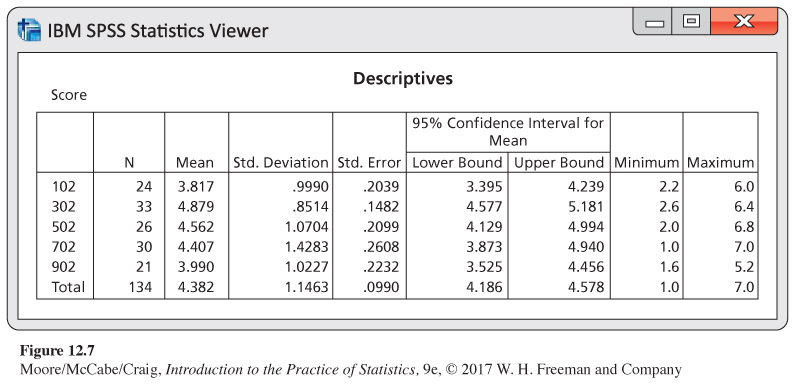
The output gives the estimates of the standard deviations, si, for each group but does not provide sp, the pooled estimate of the model standard deviation, σ. We could perform the calculation using a calculator, as we did in Example 12.6. We will see an easier way to obtain this quantity from the ANOVA table.
![]()
Some software packages report sp as part of the standard ANOVA output. Sometimes you are not sure whether or not a quantity given by software is what you think it is. A good way to resolve this dilemma is to do a sample calculation with a simple example to check the numerical results.
![]()
Note that sp is not the standard deviation given in the “Total’’ row of Figure 12.7. This quantity is the standard deviation that we would obtain if we viewed the data as a single sample of 134 participants and ignored the possibility that the profile means could be different. As we have mentioned many times before, it is important to use care when reading and interpreting software output.
EXAMPLE 12.8
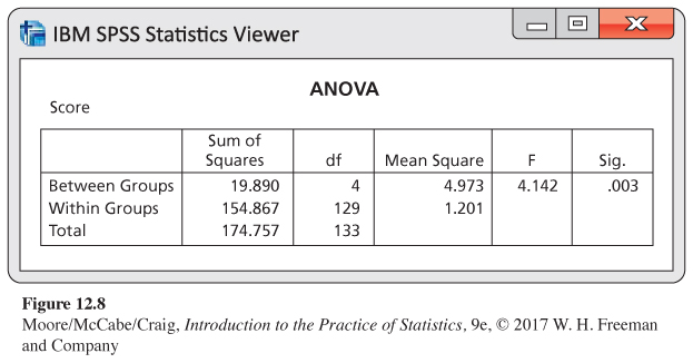
Reading software output, continued. Additional output generated by SPSS for the ANOVA of the Facebook friends example is given in Figure 12.8. We will discuss the construction of this output later. For now, we observe that the results of our significance test are given in the last two columns of the output. The null hypothesis that the five population means are the same is tested by the statistic F = 4.142, and the associated P-value is reported as P = 0.003. The data provide clear evidence to support the claim that there are some differences among the five profile population means.
The ANOVA table
The information in an analysis of variance is organized in an ANOVA table. To understand the table, it is helpful to think in terms of our
DATA = FIT + RESIDUAL
view of statistical models. For one-
xij=μi+ϵij
We can think of these three terms as sources of variation. The ANOVA table separates the variation in the data into two parts: the part due to the fit and the remainder, which we call residual.
EXAMPLE 12.9
ANOVA table for the Facebook friends study. The SPSS output in Figure 12.8 gives the sources of variation in the first column. Here, FIT is called Between Groups, RESIDUAL is called Within Groups, and DATA is the last entry, Total. Different software packages use different terms for these sources of variation but the basic concept is common to all. In place of FIT, some software packages use Between Groups, Model, or the name of the factor. Similarly, terms like Within Groups or Error are frequently used in place of RESIDUAL.
The Between Groups row in the table gives information related to the variation among group meansvariation among groups. In writing ANOVA tables, for this row we will use the generic label “groups’’ or some other term that describes the factor being studied.
The Within Groups row in the table gives information related to the variation within groupsvariation within groups. We noted that the term “error’’ is frequently used for this source of variation, particularly for more general statistical models. This label is most appropriate for experiments in the physical sciences where the observations within a group differ because of measurement error. In business and the biological and social sciences, on the other hand, the within-
Finally, the Total row in the ANOVA table corresponds to the DATA term in our DATA = FIT + RESIDUAL framework. So, for analysis of variance,
DATA = FIT + RESIDUAL
translates into
Total variation = Variation between groups + Variation within groups
sum of squares, p. 584
The second column in the software output given in Figure 12.8 is labeled Sum of Squares. As you might expect, each sum of squares is a sum of squared deviations. We use SSG, SSE, and SST for the entries in this column, corresponding to groups, error, and total. Each sum of squares measures a different type of variation. SST measures variation of the data around the overall mean, xij−ˉx. Variation of the group means around the overall mean, ˉxi−ˉx, is measured by SSG. Finally, SSE measures variation of each observation around its group mean, xij−ˉxi.
EXAMPLE 12.10
ANOVA table for the Facebook friends study, continued. The Sum of Squares column in Figure 12.8 gives the values for the three sums of squares. They are
SST = 174.757
SSG = 19.890
SSE = 154.867
Verify that SST = SSG + SSE for this example.
This fact is true in general. The total variation is always equal to the among-
In this example, it appears that most of the variation is coming from within groups. However, to assess whether the observed differences in sample means are statistically significant, some additional calculations are needed.
Associated with each sum of squares is a quantity called the degrees of freedom. Because SST measures the variation of all N observations around the overall mean, its degrees of freedom are DFT = N − 1. This is the same as the degrees of freedom for the ordinary sample variance with sample size N. Similarly, because SSG measures the variation of the I sample means around the overall mean, its degrees of freedom are DFT = I − 1. Finally, SSE is the sum of squares of the deviations xij−ˉxi. Here we have N observations being compared with I sample means, and DFE = N − I.
degrees of freedom, p. 40
EXAMPLE 12.11
Degrees of freedom for the Facebook friends study. In the Facebook friends study, we have I = 5 and N = 134. Therefore,
DFT = N − 1 = 134 − 1 = 133
DFG = I − 1 = 5 − 1 = 4
DFE = N − I = 134 − 5 = 129
These are the entries in the df column of Figure 12.8.
Note that the degrees of freedom add in the same way that the sums of squares add. That is, DFT = DFG + DFE.
For each source of variation, the mean square is the sum of squares divided by the degrees of freedom. You can verify this by doing the divisions for the values given on the output in Figure 12.8. We compare these mean squares to test whether the population means are all the same.
mean square, p. 584
SUMS OF SQUARES, DEGREES OF FREEDOM, AND MEAN SQUARES
Sums of squares represent variation present in the data. They are calculated by summing squared deviations. In one-
SST = SSG + SSE
Thus, the total variation is composed of two parts, one due to groups and one due to error.
Degrees of freedom are related to the deviations that are used in the sums of squares. The degrees of freedom are related in the same way as the sums of squares are:
DFT = DFG + DFE
To calculate each mean square, divide the corresponding sum of squares by its degrees of freedom.
We can use the mean square for error to find sp, the pooled estimate of the parameter σ of our model. It is true in general that
s2p=MSE=SSEDFE
In other words, the mean square for error is an estimate of the within-
sp=√MSE
EXAMPLE 12.12
The pooled estimate for σ. From the SPSS output in Figure 12.8 we see that the MSE is reported as 1.201. The pooled estimate of σ is therefore
sp=√MSE=√1.201=1.10
This estimate is equal to our calculations of sp in Example 12.6.
The F test
If H0 is true, there are no differences among the group means. The ratio MSG/MSE is a statistic that is approximately 1 if H0 is true and tends to be larger if Ha is true. This is the ANOVA F statistic. In our example, MSG = 4.973 and MSE = 1.201, so the ANOVA F statistic is
F=MSGMSE=4.9731.201=4.142
When H0 is true, the F statistic has an F distribution that depends upon two numbers: the degrees of freedom for the numerator and the degrees of freedom for the denominator. These degrees of freedom are those associated with the mean squares in the numerator and denominator of the F statistic. For one-
![]() The One-
The One-
The ANOVA F test shares the robustness of the two-
THE ANOVA F TEST
To test the null hypothesis in a one-
F=MSGMSE
When H0 is true, the F statistic has the F(I − 1, N − I) distribution. When Ha is true, the F statistic tends to be large. We reject H0 in favor of Ha if the F statistic is sufficiently large.
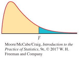
The P-value of the F test is the probability that a random variable having the F(I − 1, N − I) distribution is greater than or equal to the calculated value of the F statistic.
![]()
Tables of F critical values are available for use when software does not give the P-value. Table E in the back of the book contains the F critical values for probabilities p = 0.100, 0.050, 0.025, 0.010, and 0.001. For one-
EXAMPLE 12.13
The ANOVA F test for the Facebook friends study. In the Facebook friends study, we found F = 4.14. (Note that it is standard practice to round F statistics to two places after the decimal point.) There were five populations, so the degrees of freedom in the numerator are DFG = I − 1 = 4. For this example, the degrees of freedom in the denominator are DFE = N − I = 134 − 5 = 129. Software provided a P-value of 0.003, so at the 0.05 significance level, we reject H0 and conclude that the population means are not all the same.
| df = (4, 100) | |
|---|---|
| p | Critical value |
| 0.100 | 2.00 |
| 0.050 | 2.46 |
| 0.025 | 2.92 |
| 0.010 | 3.51 |
| 0.001 | 5.02 |
Suppose that P = 0.003 was not provided. We’ll now run through the process of using the table of F critical values to approximate the P-value. Although you will rarely need to do this in practice, the process will help you to understand the P-value calculation.
In Table E, we first find the column corresponding to 4 degrees of freedom in the numerator. For the degrees of freedom in the denominator, we see that there are entries for 100 and 200. The values for these entries are very close. To be conservative, we use critical values corresponding to 100 degrees of freedom in the denominator because these are slightly larger.
We have F = 4.14. This is in between the critical value for P = 0.010 and P = 0.001. Using the table, we can conclude only that 0.001 < P < 0.010.
The following display shows the general form of a one-
| Source | Degrees of freedom | Sum of squares | Mean square | F |
|---|---|---|---|---|
| Groups | I − 1 | ∑groupsni(ˉxi−ˉx)2 | SSG/DFG | MSG/MSE |
| Error | N − I | ∑groups(ni−1)s2i | SSE/DFE | |
| Total | N − 1 | ∑obs(xij−ˉx)2 |
One other item given by some software for ANOVA is worth noting. For an analysis of variance, we define the coefficient of determinationcoefficient of determination as
R2=SSGSST
The coefficient of determination plays the same role as the squared multiple correlation R2 in a multiple regression. We can easily calculate the value from the ANOVA table entries.
squared multiple correlation, p. 615
EXAMPLE 12.14
Coefficient of determination for the Facebook friends study. The software-
R2=SSGSST=19.890174.757=0.11
![]()
About 11% of the variation in social attractiveness scores is explained by the different profiles. The other 89% of the variation is due to participant-
USE YOUR KNOWLEDGE
Question 12.9
12.9 What’s wrong? In each of the following, identify what is wrong and then either explain why it is wrong or change the wording of the statement to make it true.
(a) Within-
group variation is the variation in the data due to the differences in the sample means. (b) The mean squares in an ANOVA table will add; that is, MST = MSG + MSE.
(c) The pooled estimate sp is a parameter of the ANOVA model.
(d) A very small P-value implies that the group distributions of responses are far apart.
12.9 (a) This sentence describes between-group variation. (b) The sums of squares in an ANOVA table will add; that is, SST = SSG + SSE. (c) σ is a parameter, not sp. (d) A small P means the means are not all the same, but the distributions may still overlap quite a bit.
Question 12.10
12.10 Determining the critical value of F. For each of the following situations, state how large the F statistic needs to be for rejection of the null hypothesis at the 0.05 level.
(a) Compare three groups with four observations per group.
(b) Compare three groups with five observations per group.
(c) Compare four groups with five observations per group.
(d) Summarize what you have learned about F distributions from this exercise.
Software
We have used SPSS to illustrate the analysis of the Facebook friends study. Other statistical software gives similar output, and you should be able to read it without any difficulty. Here’s an example with output from three software packages.
EXAMPLE 12.15
Do eyes affect ad response? Research from a variety of fields has found significant effects of eye gaze and eye color on emotions and perceptions such as arousal, attractiveness, and honesty. These findings suggest that a model’s eyes may play a role in a viewer’s response to an ad.

In one study, students in marketing and management classes of a southern, predominantly Hispanic, university were each presented with one of four portfolios.4 Each portfolio contained a target ad for a fictional product, Sparkle Toothpaste. Students were asked to view the ad and then respond to questions concerning their attitudes and emotions about the ad and product. All questions were from advertising-
Although the researchers investigated nine attitudes and emotions, we will focus on the viewer’s “attitudes toward the brand.’’ This response was obtained by averaging 10 survey questions.
The target ads were created using two digital photographs of a model. In one picture, the model is looking directly at the camera so the eyes can be seen. This picture was used in three target ads. The only difference was the model’s eyes, which were made to be either brown, blue, or green. In the second picture, the model is in virtually the same pose but looking downward so the eyes are not visible. A total of 222 surveys were used for analysis. Outputs from Excel, SAS, and Minitab are given in Figure 12.9.
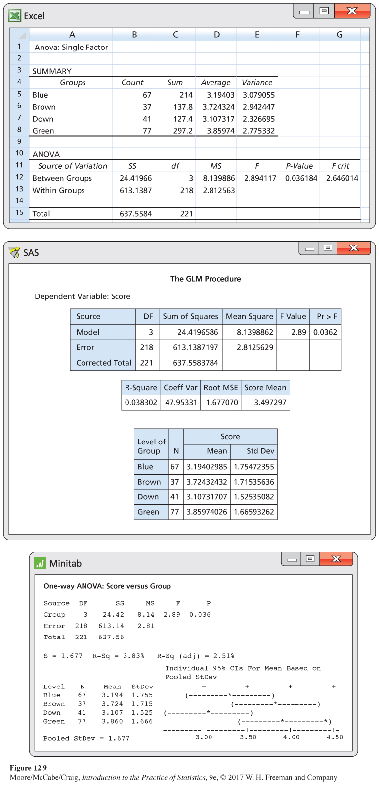
There is evidence at the 5% significance level to reject the null hypothesis that the four groups have equal means (P = 0.036). In Exercises 12.35 and 12.36 (page 686), you are asked to perform further inference using contrasts.
BEYOND THE BASICS
Testing the Equality of Spread
While the standard deviation is a natural measure of spread for Normal distributions, it is not for distributions in general. In fact, because skewed distributions have unequally spread tails, no single numerical measure is adequate to describe the spread of a skewed distribution. Because of this, we recommend caution when testing equal standard deviations and interpreting the results.
Most formal tests for equal standard deviations are extremely sensitive to non-
MODIFIED LEVENE’S TEST FOR EQUALITY OF STANDARD DEVIATIONS
To test for the equality of the I population standard deviations, perform a one-
yij=|xij−Mi|
where Mi is the sample median for population i. We reject the assumption of equal spread if the P-value of this test is less than the significance level ⍺.
This test uses a more robust measure of deviation replacing the mean with the median and replacing squaring with the absolute value. Also, the transformed response variable is straightforward to create, so this test can easily be performed regardless of whether or not your software specifically has it.
EXAMPLE 12.16
Are the Standard Deviations Equal? Figure 12.10 shows output of the modified Levene’s test for the Facebook friends study. In JMP, the test is called Brown-
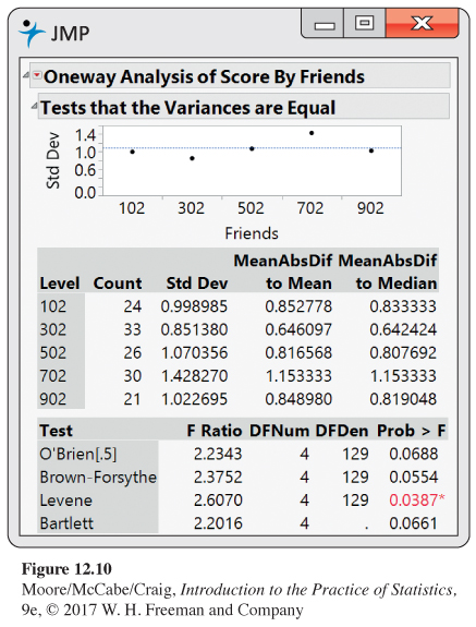
![]()
Remember that our rule of thumb (page 654) is used to assess whether different standard deviations will impact the ANOVA results. It’s not a formal test that the standard deviations are equal. There will be times when the rule and formal test do not agree.