Chapter 12: One-Way Analysis of Variance

12.2 12.2 Comparing the Means

670

When you complete this section, you will be able to:

• Distinguish between the use of contrasts to examine particular versions of the alternative hypothesis and the use of a multiple-comparisons method to compare pairs of means.
• Construct a level C confidence interval for a comparison of means expressed as a contrast.
• Perform a t significance test for a contrast and summarize the results.
• Summarize the trade-off of a multiple-comparisons method in terms of controlling false rejections and not detecting true differences in means.
• Describe and use the Bonferroni method to control the probability of a false rejection.
• Interpret statistical software ANOVA output and draw conclusions regarding differences in population means.
• Determine the power of the ANOVA F test for a given set of population means and sample sizes.

The ANOVA F test gives a general answer to a general question: are the differences among observed group means statistically significant? Unfortunately, a small P-value simply tells us that the group means are not all the same. It does not tell us specifically which means differ from each other. Plotting and inspecting the means give us some indication of where the differences lie, but we would like to supplement inspection with formal inference. This section presents two approaches to the task of comparing group means.

Contrasts

In the ideal situation, specific questions regarding comparisons among the means are posed before the data are collected. We can answer specific questions of this kind and attach a level of confidence to the answers we give. We now explore these ideas through a different Facebook study.

EXAMPLE 12.17

How do users spend their time on Facebook? An online study was designed to compare the amount of time a Facebook user devotes to reading positive, negative, and neutral Facebook profiles. Each participant was randomly assigned to one of five Facebook profile groups:

1. Positive female
2. Positive male
3. Negative female
4. Negative male
5. Gender neutral with neutral content

671

and provided an email link to a survey on Survey Monkey. As part of the survey, the participant was directed to view the assigned Facebook profile page and then answer some additional questions. The amount of time (in minutes) the participant spent viewing the profile was recorded as the response.⁷

We begin our analysis with a check of the data. Time-to-event data (here, the time until the participant begins to answer the additional survey questions) is often skewed to the right. Preliminary analysis of the residuals (Figure 12.11) confirms this for these data.

Figure 12.11: FIGURE 12.11 Normal quantile plot of residuals suggests a skewed distribution, Example 12.17.

Figure 12.12: FIGURE 12.12 SPSS output giving the ANOVA table for the Facebook profile study after the square root transformation, Example 12.17.

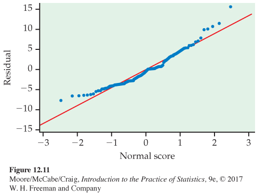
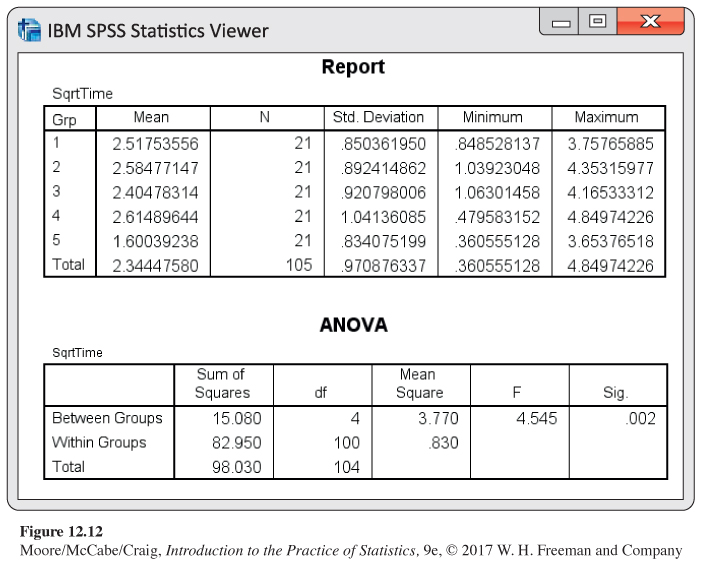
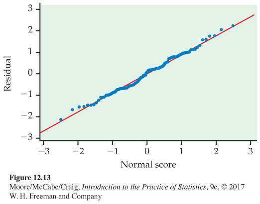
As a result, we consider the square root of time for analysis. These results are summarized in Figure 12.12 and 12.13. The residuals appear Normal (Figure 12.13), and our rule for examining standard deviations indicates we can assume equal population standard deviations (1.041 < 2(0.834)). The F test is significant with a P-value of 0.002. It’s testing the null hypothesis

672

Figure 12.13: FIGURE 12.13 Normal quantile plot of residuals for the transformed response, Example 12.17.

H₀: μ₁ = μ₂ = μ₃ = μ₄ = μ₅

versus the alternative that the five population means are not all the same. Because the P-value is very small, there is strong evidence against H₀ and we can conclude that the five population means are not all the same (F(4,100) = 4.55 with P = 0.002).

However, having evidence that the five population means are not the same does not tell us all we’d like to know. We would really like our analysis to provide us with more specific information. For example, the alternative hypothesis is true if

μ₁ < μ₂ = μ₃ = μ₄ = μ₅

or if

μ₁ = μ₂ > μ₃ = μ₄ > μ₅

or if

μ₁ < μ₃ < μ₄ < μ₂ < μ₅

When you reject the ANOVA null hypothesis, additional analyses are required to clarify the nature of the differences between the means.

For this study, the researcher predicted that participants would spend more time viewing the negative Facebook pages compared to the positive or neutral pages because the negative pages would stand out more and thus garner more attention (this is called cognitive salience). How do we take these predictions and translate them into testable hypotheses?

EXAMPLE 12.18

A comparison of interest. The researcher hypothesizes that participants exposed to a negative Facebook profile would spend more time viewing the page than would participants who are exposed to a positive Facebook profile. Because two groups are exposed to negative profiles and two are exposed to positive profiles, we can consider the following null hypothesis:

673

versus the two-sided alternative

We could argue that the one-sided alternative

is appropriate for this problem provided other evidence suggests this direction and is not just what the researcher wants to see.

In the preceding example, we used H₀₁ and H_a₁ to designate the null and alternative hypotheses. The reason for this is that there is an additional set of hypotheses to assess. We use H₀₂ and H_a₂ for this set.

EXAMPLE 12.19

Another comparison of interest. This comparison tests if there is a difference in time between groups exposed to a negative page and the group exposed to the neutral page. Here are the null and alternative hypotheses:

Each of H₀₁ and H₀₂ says that a combination of population means is 0. These combinations of means are called contrasts because the coefficients sum to zero. We use ψ, the Greek letter psi, for contrasts among population means. For our first comparison, we have

and for the second comparison

In each case, the value of the contrast is 0 when H₀ is true. Note that we have chosen to define the contrasts so that they will be positive when the alternative of interest (what we expect) is true. Whenever possible, this is a good idea because it makes some computations easier.

A contrast expresses an effect in the population as a combination of population means. To estimate the contrast, form the corresponding sample contrastsample contrast by using sample means in place of population means. Under the ANOVA assumptions, a sample contrast is a linear combination of independent Normal variables and, therefore, has a Normal distribution (page 304). We can obtain the standard error of a contrast by using the rules for variances. Inference is based on t statistics. Here are the details.

rules for variances, p. 258

674

CONTRASTS

A contrast is a combination of population means of the form

where the coefficients a_i sum to 0. The corresponding sample contrast is

The standard error of c is

To test the null hypothesis

H₀: ψ = 0

use the t statistic

with degrees of freedom DFE that are associated with s_p. The alternative hypothesis can be one-sided or two-sided.

A level C confidence interval for c is

c ± t*SE_c

where t* is the value for the t(DFE) density curve with area C between −t* and t*.

Because each estimates the corresponding μ_i, the addition rule for means tells us that the mean μ_c of the sample contrast c is ψ. In other words, c is an unbiased estimator of ψ. Testing the hypothesis that a contrast is 0 assesses the significance of the effect measured by the contrast. It is often more informative to estimate the size of the effect using a confidence interval for the population contrast.

addition rule for means, p. 254

EXAMPLE 12.20

The contrast coefficients. In our example the coefficients in the contrasts are

a₁ = −0.5, a₂ = −0.5, a₃ = 0.5, a₄ = 0.5, a₅ = 0, for ψ₁

and

a₁ = 0, a₂ = 0, a₃ = 0.5, a₄ = 0.5, a₅ = −1, for ψ₂

where the subscripts 1, 2, 3, 4, and 5 correspond to the profiles listed in Example 12.17, respectively. In each case the sum of the a_i is 0. We look at inference for each of these contrasts in turn.

675

EXAMPLE 12.21

Testing the first contrast of interest. The sample contrast that estimates ψ₁ is

with standard error

= 0.1988

The t statistic for testing H₀₁: ψ₁ = 0 versus H_a₁: ψ₁ > 0 is

Because s_p has 100 degrees of freedom, software using the t(100) distribution gives the two-sided P-value as P = 0.8341. If we used Table D, we would conclude that P > 2(0.25) = 0.50. The P-value is very large, so there is little evidence against H₀₁.

We use the same method for the second contrast.

EXAMPLE 12.22

Testing the second contrast of interest. The sample contrast that estimates ψ2 is

= (0.5)2.405 + (0.5)2.615 + (−1)1.600

= 1.2025 + 1.3075 − 1.600

= 0.91

with standard error

= 0.2435

The t statistic for assessing the significance of this contrast is

The P-value for the two-sided alternative is 0.0003. If we used Table D, we would conclude that P < 2(0.0005) = 0.001. The P-value is very small, so there is strong evidence against H₀₂.

We have strong evidence to conclude that time viewing a negative content page is different from the time viewing a neutral content page. The size of the difference can be described with a confidence interval.

676

EXAMPLE 12.23

Confidence interval for the second contrast. To find the 95% confidence interval for ψ₂, we combine the estimate with its margin of error:

= 0.91 ± 0.47

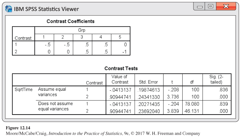
The interval is (0.44, 1.38). Unfortunately, this interval is difficult to interpret because the units are . We can obtain an approximate 95% interval on the orginial units scale by back-transforming (squaring the interval end points). This results in an approximate 95% confidence interval of the difference to be between 0.19 minutes and 1.90 minutes.

SPSS output for the contrasts is given in Figure 12.14. The results agree with the calculations that we performed in Examples 12.21 and 12.22 except for minor differences due to roundoff error in our calculations. Note that the output does not give the confidence interval that we calculated in Example 12.23. This is easily computed, however, from the contrast estimate and standard error provided in the output.

Some statistical software packages report the test statistics associated with contrasts as F statistics rather than t statistics. These F statistics are the squares of the t statistics described previously. As with much statistical software output, P-values for significance tests are reported for the two-sided alternative.

If the software you are using gives P-values for the two-sided alternative, and you are using the appropriate one-sided alternative, divide the reported P-value by 2. In our example, we argued that a one-sided alternative may be appropriate for the first contrast. The software reported the P-value as 0.836, so we can conclude P = 0.418. Dividing this value by 2 has no effect on the conclusion.

Questions about population means are expressed as hypotheses about contrasts. A contrast should express a specific question that we have in mind when designing the study. Because the ANOVA F test answers a very general question, it is less powerful than tests for contrasts designed to answer specific questions.

Figure 12.14: FIGURE 12.14 SPSS output giving the contrast analysis for the Facebook profile study (Example 12.17).

677

When contrasts are formulated before seeing the data, inference about contrasts is valid whether or not the ANOVA H₀ of equality of means is rejected. Specifying the important questions before the analysis is undertaken enables us to use this powerful statistical technique.

USE YOUR KNOWLEDGE

Question 12.27

12.27 Defining a contrast. Refer to Example 12.17 (page 670). Suppose the researcher was also interested in comparing the viewing time between male and female profile pages. Specify the coefficients for this contrast.

Question 12.28

12.28 Defining different coefficients. Refer to Example 12.22 (page 675). Suppose we had selected the coefficients a₁ = 0, a₂ = 0, a₃ = −1, a₄ = −1, and a₅ = 2. Would this choice of coefficients alter our inference in this example? Explain your answer.

Multiple comparisons

In many studies, specific questions cannot be formulated in advance of the analysis. If H₀ is not rejected, we conclude that the population means are indistinguishable on the basis of the data given. On the other hand, if H₀ is rejected, we would like to know which pairs of means differ. Multiple-comparisons methodsmultiple-comparisons methods address this issue. It is important to keep in mind that multiple-comparisons methods are used only after rejecting the ANOVA H₀.

EXAMPLE 12.24

Comparing each pair of groups. Let’s return once more to the Facebook friends data with five groups (page 648). We can make 10 comparisons between pairs of means. We can write a t statistic for each of these pairs. For example, the statistic

= −3.59

compares profiles with 102 and 302 friends. The subscripts on t specify which groups are compared.

The t statistics for two other pairs are

= 1.11

= 2.90

678

These 10 t statistics are very similar to the pooled two-sample t statistic for comparing two population means. The difference is that we now have more than two populations, so each statistic uses the pooled estimator s_p from all groups rather than the pooled estimator from just the two groups being compared. This additional information about the common σ increases the power of the tests. The degrees of freedom for all these statistics are , those associated with .

two-sample t procedures, p. 449

Because we do not have any specific ordering of the means in mind as an alternative to equality, we must use a two-sided approach to the problem of deciding which pairs of means are significantly different.

MULTIPLE COMPARISONS

To perform a multiple-comparisons procedure, compute t statistics for all pairs of means using the formula

we declare that the population means μ_i and μ_j are different. Otherwise, we conclude that the data do not distinguish between them. The value of t** depends upon which multiple-comparisons procedure we choose.

One obvious choice for t** is the upper ⍺/2 critical value for the t(DFE) distribution. This choice simply carries out as many separate significance tests of fixed level ⍺ as there are pairs of means to be compared. The procedure based on this choice is called the least-significant differences methodLSD method, or simply LSD.

LSD has some undesirable properties, particularly if the number of means being compared is large. Suppose, for example, that there are I = 20 groups and we use LSD with ⍺ = 0.05. There are 190 different pairs of means. If we perform 190 t tests, each with an error rate of 5%, our overall error rate will be unacceptably large. We expect about 5% of the 190 to be significant even if the corresponding population means are the same. Because 5% of 190 is 9.5, we expect 9 or 10 false rejections.

The LSD procedure fixes the probability of a false rejection for each single pair of means being compared. It does not control the overall probability of some false rejection among all pairs. Other choices of t** control possible errors in other ways. The choice of t** is, therefore, a complex problem, and a detailed discussion of it is beyond the scope of this text. Many choices for t** are used in practice. Most statistical packages provide several to choose from.

Bonferroni procedure, p. 391

We will discuss only one of these, called the Bonferroni method. Use of this procedure with ⍺ = 0.05, for example, guarantees that the probability of any false rejection among all comparisons made is no greater than 0.05. This is much stronger protection than controlling the probability of a false rejection at 0.05 for each separate comparison.

679

EXAMPLE 12.25

Applying the Bonferroni method. We apply the Bonferroni multiple-comparisons procedure with ⍺ = 0.05 to the data from the Facebook friends study. Given 10 comparisons of interest, the value of t** for this procedure uses ⍺ = 0.05/10 = 0.005 for each test. From Table D, this value is 2.63. Of the statistics t₁₂ = −3.59, t₂₃ = 1.11, and t₂₅ = 2.90 calculated in Example 12.24, only t₁₂ and t₂₅ are significant. These two statistics compare the profile of 302 friends with the two extreme levels.

Of course, we prefer to use software for the calculations.

EXAMPLE 12.26

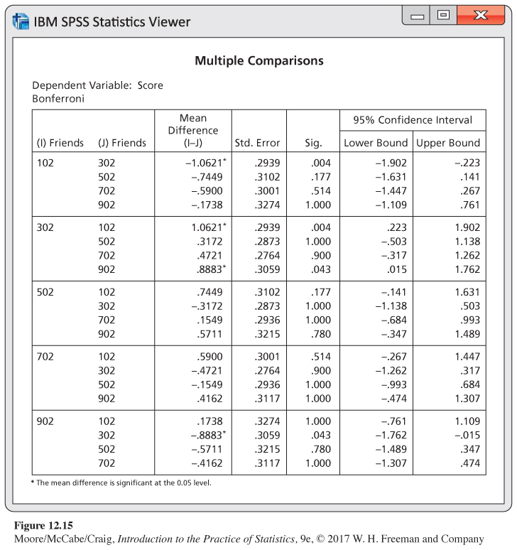
Interpreting software output. The output generated by SPSS for Bonferroni comparisons appears in Figure 12.15. The software uses an asterisk to indicate that the difference in a pair of means is statistically significant. Here, all 10 comparisons are reported. These results agree with the calculations that we performed in Examples 12.24 and 12.25. There are no significant differences except those already mentioned. Note that each comparison is given twice in the output.

The data in the Facebook friends study provide a clear result: the social attractiveness score increases as the number of friends increases to a point and then decreases. Unfortunately with these data, we cannot accurately describe this relationship in more detail. This lack of clarity is not unusual when performing a multiple-comparisons analysis.

Here, the mean associated with 302 friends is significantly different from the means for the 102- and 902-friend profiles, but it is not found significantly different from the means for the profiles with 502 and 702 friends. To complicate things, the means for profiles with 502 and 702 friends were not found significantly different from the means for the 102- and 902-friend profiles.

This kind of apparent contradiction points out dramatically the nature of the conclusions of statistical tests of significance. The conclusion appears to be illogical. If μ₁ is the same as μ₃ and if μ₃ is the same as μ₂, doesn’t it follow that μ₁ is the same as μ₂? Logically, the answer must be Yes.

Some of the difficulty can be resolved by noting the choice of words used. In describing the inferences, we talk about failing to detect a difference or concluding that two groups are different. In making logical statements, we say things such as “is the same as.’’ There is a big difference between the two modes of thought. Statistical tests ask, “Do we have adequate evidence to distinguish two means?’’ It is not illogical to conclude that we have sufficient evidence to distinguish μ₁ from μ₂, but not μ₁ from μ₃ or μ₂ from μ₃.

One way to deal with these difficulties of interpretation is to give confidence intervals for the differences. The intervals remind us that the differences are not known exactly. We want to give simultaneous confidence intervals, that is, intervals for all differences among the population means at once. Again, we must face the problem that there are many competing procedures—in this case, many methods of obtaining simultaneous intervals.

680

Figure 12.15: FIGURE 12.15 SPSS output giving the multiple-comparisons analysis for the Facebook friends study, Example 12.26.

SIMULTANEOUS CONFIDENCE INTERVALS FOR DIFFERENCES BETWEEN MEANS

Simultaneous confidence intervals for all differences μ_i − μ_j between population means have the form

The critical values t** are the same as those used for the multiple-comparisons procedure chosen.

The confidence intervals generated by a particular choice of t** are closely related to the multiple-comparisons results for that same method. If one of the confidence intervals includes the value 0, then that pair of means will not be declared significantly different, and vice versa.

681

EXAMPLE 12.27

Interpreting software output, continued. The SPSS output for the Bonferroni multiple-comparisons procedure given in Figure 12.15 includes the simultaneous 95% confidence intervals. We can see, for example, that the interval for μ₁ − μ₃ is −1.63 to 0.14. The fact that the interval includes 0 is consistent with the fact that we failed to detect a difference between these two means using this procedure. Note that the interval for μ₃ − μ₁ is also provided. This is not really a new piece of information because it can be obtained from the other interval by reversing the signs and reversing the order, that is, –0.14 to 1.63. So, in fact, we really have only 10 intervals. Use of the Bonferroni procedure provides us with 95% confidence that all 10 intervals simultaneously contain the true values of the population mean differences.

USE YOUR KNOWLEDGE

Question 12.29

12.29 Why no multiple comparisons? Any pooled two-sample t problem can be run as a one-way ANOVA with I = 2. Explain why it is inappropriate to analyze the data using multiple-comparisons procedures in this setting.

Question 12.30

12.30 Growth of Douglas fir seedlings. An experiment was conducted to compare the growth of Douglas fir seedlings under three different levels of vegetation control (0%, 50%, and 100%). Sixteen seedlings were randomized to each level of control. The resulting sample means for stem volume were 58, 73, and 105 cubic centimeters (cm³), respectively, with s_p = 17 cm³. The researcher hypothesized that the average growth at 50% control would be less than the average of the 0% and 100% levels.

(a) What are the coefficients for testing this contrast?
(b) Perform the test and report the test statistic, degrees of freedom, and P-value. Do the data provide evidence to support this hypothesis?

Power

Recall that the power of a test is the probability of rejecting H₀ when H_a is, in fact, true. Power measures how likely a test is to detect a specific alternative. When planning a study in which ANOVA will be used for the analysis, it is important to perform power calculations to check that the sample sizes are adequate to detect differences among means that are judged to be important.

Power calculations also help evaluate and interpret the results of studies in which H₀ was not rejected. We sometimes find that the power of the test was so low against reasonable alternatives that there was little chance of obtaining a significant F.

power, p. 392

In Chapter 7, we found the power for the two-sample t test. One-way ANOVA is a generalization of the two-sample t test, so it is not surprising that the procedure for calculating power is quite similar.

Here are the steps that are needed:

682

1. Specify
1. (a) An alternative (H_a) that you consider important; that is, values for the true population means μ₁, μ₂, . . . , μ_I.
2. (b) Sample sizes n₁, n₂, . . . , n_I; usually these will all be equal to the common value n.
3. (c) A level of significance ⍺, usually equal to 0.05.
4. (d) A guess at the standard deviation σ.
2. Use the degrees of freedom DFG = I − 1 and DFE = N − I to find the critical value that will lead to the rejection of H₀. This value, which we denote by F*, is the upper ⍺ critical value for the F(DFG,DFE) distribution.
3. Calculate the noncentrality parameternoncentrality parameter⁸

where is a weighted average of the group means

If the means are all equal (the ANOVA H₀), then λ = 0. The noncentrality parameter measures how unequal the given set of means is. Large λ points to an alternative far from H₀, and we expect the ANOVA F test to have high power.

4. Find the power, which is the probability of rejecting H₀ when the alternative hypothesis is true; that is, the probability that the observed F is greater than F*. Under H_a, the F statistic has a distribution known as the noncentral F distribution. SAS, for example, has a function for this distribution. Using this function, the power is

noncentral F distribution

Power = 1 − PROBF (F*, DFG, DFE, λ)

Software makes calculation of the power quite easy. The software does Steps 2, 3, and 4, so our task simplifies to just Step 1. Some software doesn’t request the alternative means, but rather a difference in means that is judged important. Most software will also assume a constant sample size. Let’s run through an example doing the calculations ourselves and then compare the results with output from two software programs.

EXAMPLE 12.28

Power of a reading comprehension study. Suppose that a study on reading comprehension for three different teaching methods has 10 students in each group. How likely is this study to detect differences in the mean responses? A previous study performed in a different setting found sample means of 41, 47, and 44, and the pooled standard deviation was 7. Based on these results, we will use μ₁ = 41, μ₂ = 47, μ₃ = 44, and σ = 7 in a calculation of power. The n_i are equal, so is simply the average of the :

683

The noncentrality parameter is, therefore,

Because there are three groups with 10 observations per group, DFG = 2 and DFE = 27. The critical value for ⍺ = 0.05 is F* = 3.35. The power is, therefore,

1 − PROBF(3.35, 2, 27, 3.67) = 0.3486

The chance that we reject the ANOVA H₀ at the 5% significance level given these population means and standard deviation is slightly less than 35%.

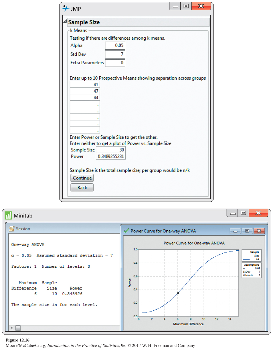
Figure 12.16: FIGURE 12.16 JMP and Minitab power calculation outputs, Example 12.28.

Figure 12.16 shows the power calculation output from JMP and Minitab. For JMP, you specify the alternative means, standard deviation, and the total sample size N. The power is calculated once the “Continue’’ button is clicked. Notice that this result is the same as the result in Example 12.28. For Minitab, you enter the common sample size n, standard deviation σ, and the difference between means that is deemed important. For the alternative means specified in Example 12.28, the largest difference is 6 = 47 − 41, so that was entered. The power is again the same as the result in Example 12.28. This won’t always be the case. Specifying an important difference will often give a power value that is smaller. This is because it computes a noncentrality parameter that is always less than or equal to the noncentrality value based on knowing all the alternative means.

684

If the assumed values of the μ_i in this example describe differences among the groups that the experimenter wants to detect, then we would want to use more than 10 subjects per group. Although H₀ is false for these μ_i, the chance of rejecting it at the 5% level is only about 35%. This chance can be increased to acceptable levels by increasing the sample sizes.

EXAMPLE 12.29

Changing the sample size. To decide on an appropriate sample size for the experiment described in the previous example, we repeat the power calculation for different values of n, the number of subjects in each group. Here are the results:

n	DFG	DFE	F*	l	Power
20	2	57	3.16	7.35	0.65
30	2	87	3.10	11.02	0.84
40	2	117	3.07	14.69	0.93
50	2	147	3.06	18.37	0.97
100	2	297	3.03	36.73	͌1

685

Try using JMP to verify these calculations. With n = 40, the experimenters have a 93% chance of rejecting H₀ with ⍺ = 0.05 and thereby demonstrating that the groups have different means. In the long run, 93 out of every 100 such experiments would reject H₀ at the ⍺ = 0.05 level of significance. Using 50 subjects per group increases the chance of finding significance to 97%. With 100 subjects per group, the experimenters are virtually certain to reject H₀. The exact power for n = 100 is 0.99990. In most real-life situations, the additional cost of increasing the sample size from 50 to 100 subjects per group would not be justified by the relatively small increase in the chance of obtaining statistically significant results.

USE YOUR KNOWLEDGE

Question 12.31

12.31 Understanding power calculations. Refer to Example 12.28. Suppose that the researcher decided to use μ₁ = 39, μ₂ = 44, and μ₃ = 49 in the power calculations. With n = 10 and σ = 7, would the power be larger or smaller than 35%? Explain your answer.

Question 12.32

12.32 Understanding power calculations, continued. If all the group means are equal (H₀ is true), what is the power of the F test? Explain your answer.