4.2 4.2 Probability Models
When you complete this section, you will be able to:
• Describe a sample space from a description of a random phenomenon.
• Apply the four probability rules.
• Identify random phenomena that have equally likely outcomes and distinguish them from those that do not.
The idea of probability as a proportion of outcomes in very many repeated trials guides our intuition but is hard to express in mathematical form. A description of a random phenomenon in the language of mathematics is called a probability modelprobability model. To see how to proceed, think first about a very simple random phenomenon, tossing a coin once. When we toss a coin, we cannot know the outcome in advance. What do we know? We are willing to say that the outcome will be either heads or tails. Because the coin appears to be balanced, we believe that each of these outcomes has probability 1/2. This description of coin tossing has two parts:
• A list of possible outcomes.
• A probability for each outcome.
This two-part description is the starting point for a probability model. We will begin by describing the outcomes of a random phenomenon and then learn how to assign probabilities to the outcomes.
Sample spaces
A probability model first tells us what outcomes are possible.
SAMPLE SPACE
The sample space S of a random phenomenon is the set of all possible outcomes.
The name “sample space” is natural in random sampling, where each possible outcome is a sample and the sample space contains all possible samples. To specify S, we must state what constitutes an individual outcome and then state which outcomes can occur. We often have some freedom in defining the sample space, so the choice of S is a matter of convenience as well as correctness. The idea of a sample space, and the freedom we may have in specifying it, are best illustrated by examples.
EXAMPLE 4.4
Sample space for tossing a coin. Toss a coin. There are only two possible outcomes, and the sample space is
S = {heads, tails}
or, more briefly, S = {H, T}.
EXAMPLE 4.5
Sample space for random digits. Let your pencil point fall blindly into Table B of random digits. Record the value of the digit it lands on. The possible outcomes are
S = {0, 1, 2, 3, 4, 5, 6, 7, 8, 9}
EXAMPLE 4.6
Sample space for tossing a coin four times. Toss a coin four times and record the results. That’s a bit vague. To be exact, record the results of each of the four tosses in order. A typical outcome is then HTTH. Counting shows that there are 16 possible outcomes. The sample space S is the set of all 16 strings of four H’s and T’s.
Suppose that our only interest is the number of heads in four tosses. Now we can be exact in a simpler fashion. The random phenomenon is to toss a coin four times and count the number of heads. The sample space contains only five outcomes:
S = {0, 1, 2, 3, 4}
This example illustrates the importance of carefully specifying what constitutes an individual outcome.
Although these examples seem remote from the practice of statistics, the connection is surprisingly close. Suppose that in conducting an opinion poll you select four people at random from a large population and ask each if he or she favors reducing federal spending on low-interest student loans. The answers are Yes or No. The possible outcomes—the sample space—are exactly as in Example 4.6 if we replace heads by Yes and tails by No. Similarly, the possible outcomes of an SRS of 1500 people are the same, in principle, as the possible outcomes of tossing a coin 1500 times. One of the great advantages of mathematics is that the essential features of quite different phenomena can be described by the same probability model.
USE YOUR KNOWLEDGE
Question 4.8
4.8 When were you born? A student is asked “In what month were you born? Set up an appropriate sample space for this setting.
The sample spaces described in Examples 4.4, 4.5, and 4.6 correspond to categorical variables where we can list all the possible values. Other sample spaces correspond to quantitative variables. Here is an example.
EXAMPLE 4.7
Using software. Most statistical software has a function that will generate a random number between 0 and 1. The sample space is
S = {all numbers between 0 and 1}
This S is a mathematical idealization. Any specific random number generator produces numbers with some limited number of decimal places so that, strictly speaking, not all numbers between 0 and 1 are possible outcomes. For example, Minitab generates random numbers like 0.736891, with six decimal places. The entire interval from 0 to 1 is easier to think about. It also has the advantage of being a suitable sample space for different software systems that produce random numbers with different numbers of digits.
USE YOUR KNOWLEDGE

Question 4.9
4.9 How many hours do you text? You record the number of hours per week that a randomly selected student spends texting. What is the sample space?
4.9 S = {all numbers between 0 and 168}.
A sample space S lists the possible outcomes of a random phenomenon. To complete a mathematical description of the random phenomenon, we must also give the probabilities with which these outcomes occur.
The true long-term proportion of any outcome—say, “exactly two heads in four tosses of a coin”—can be found only empirically, and then only approximately. How then can we describe probability mathematically? Rather than immediately attempting to give “correct” probabilities, let’s confront the easier task of laying down rules that any assignment of probabilities must satisfy. We need to assign probabilities not only to single outcomes but also to sets of outcomes.
EVENT
An event is an outcome or a set of outcomes of a random phenomenon. That is, an event is a subset of the sample space.
EXAMPLE 4.8
Exactly one head in four tosses. Take the sample space S for four tosses of a coin to be the 16 possible outcomes in the form HTHH. Then “exactly one head” is an event. Call this event A. The event A expressed as a set of outcomes is
A = {HTTT, THTT, TTHT, TTTH}
In a probability model, events have probabilities. What properties must any assignment of probabilities to events have? Here are some basic facts about any probability model. These facts follow from the idea of probability as “the long-run proportion of repetitions on which an event occurs.”
1. Any probability is a number between 0 and 1. Any proportion is a number between 0 and 1, so any probability is also a number between 0 and 1. An event with probability 0 never occurs, and an event with probability 1 occurs on every trial. An event with probability 0.5 occurs in half the trials in the long run.
2. All possible outcomes together must have probability 1. Because every trial will produce an outcome, the sum of the probabilities for all possible outcomes must be exactly 1.
3. If two events have no outcomes in common, the probability that one or the other occurs is the sum of their individual probabilities. If one event occurs in 40% of all trials, a different event occurs in 25% of all trials, and the two can never occur together, then one or the other occurs in 65% of all trials because 40% + 25% = 65%.
4. The probability that an event does not occur is 1 minus the probability that the event does occur. If an event occurs in (say) 70% of all trials, it fails to occur in the other 30%. The probability that an event occurs and the probability that it does not occur always add to 100%, or 1.
Probability rules
Formal probability uses mathematical notation to state Facts 1 through 4 more concisely. We use capital letters near the beginning of the alphabet to denote events. If A is any event, we write its probability as P(A). Here are our probability facts in formal language. As you apply these rules, remember that they are just another form of intuitively true facts about long-run proportions.
PROBABILITY RULES
Rule 1. The probability P(A) of any event A satisfies 0 ≤ P(A) ≤ 1.
Rule 2. If S is the sample space in a probability model, then P(S) = 1.
Rule 3. Two events A and B are disjoint if they have no outcomes in common and so can never occur together. If A and B are disjoint,
P(A or B) = P(A) + P(B)
This is the addition rule for disjoint events.
Rule 4. The complement of any event A is the event that A does not occur, written as Ac. The complement rule states that
P(Ac) = 1 − P(A)
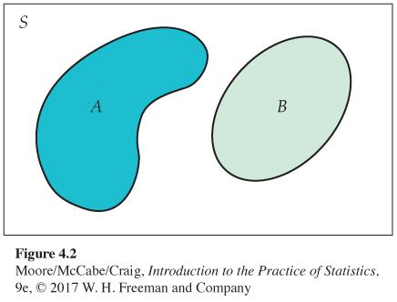
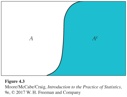
You may find it helpful to draw a picture to remind yourself of the meaning of complements and disjoint events. A picture like Figure 4.2 that shows the sample space S as a rectangular area and events as areas within S is called a Venn diagramVenn diagram. The events A and B in Figure 4.2 are disjoint because they do not overlap. As Figure 4.3 shows, the complement Ac contains exactly the outcomes that are not in A.
EXAMPLE 4.9
Favorite vehicle colors. What is your favorite color for a vehicle? Our preferences can be related to our personality, our moods, or particular objects. Here is a probability model for color preferences.2

| Color | White | Black | Silver | Gray |
| Probability | 0.24 | 0.19 | 0.16 | 0.15 |
| Color | Red | Blue | Brown | Other |
| Probability | 0.10 | 0.07 | 0.05 | 0.04 |
Each probability is between 0 and 1. The probabilities add to 1 because these outcomes together make up the sample space S. Our probability model corresponds to selecting a person at random and asking what is their favorite color.
Let’s use the probability Rules 3 and 4 to find some probabilities for favorite vehicle colors.
EXAMPLE 4.10
Black or silver? What is the probability that a person’s favorite vehicle color is black or silver? If the favorite is black, it cannot be silver, so these two events are disjoint. Using Rule 3, we find
P(black or silver)=P(black)+P(silver)=0.19+0.16=0.35
There is a 35% chance that a randomly selected person will choose black or silver as their favorite color. Suppose that we want to find the probability that the favorite color is not blue.
EXAMPLE 4.11
Use the complement rule. To solve this problem, we could use Rule 3 and add the probabilities for white, black, silver, gray, red, brown and other. However, it is easier to use the probability that we have for blue and Rule 4. The event that the favorite is not blue is the complement of the event that the favorite is blue. Using our notation for events, we have
P(not blue)=1-P(blue)=1-0.07=0.93
We see that 93% of people have a favorite vehicle color that is not blue.
USE YOUR KNOWLEDGE
Question 4.10
4.10 Red or brown. Find the probability that the favorite color is red or brown.
Question 4.11
4.11 White, black, silver, gray, or red. Find the probability that the favorite color is white, black, silver, gray, or red using Rule 4. Explain why this calculation is easier than finding the answer using Rule 3.
4.11 0.84. Adding three probabilities and subtracting that result from 1 is slightly easier than adding the five probabilities of interest.
Assigning probabilities: Finite number of outcomes
The individual outcomes of a random phenomenon are always disjoint. So the addition rule provides a way to assign probabilities to events with more than one outcome: start with probabilities for individual outcomes and add to get probabilities for events. This idea works well when there are only a finite (fixed and limited) number of outcomes.
PROBABILITIES IN A FINITE SAMPLE SPACE
Assign a probability to each individual outcome. These probabilities must be numbers between 0 and 1 and must have sum 1.
The probability of any event is the sum of the probabilities of the outcomes making up the event.
EXAMPLE 4.12
Benford’s law. Faked numbers in tax returns, payment records, invoices, expense account claims, and many other settings often display patterns that aren’t present in legitimate records. Some patterns, such as too many round numbers, are obvious and easily avoided by a clever crook. Others are more subtle. It is a striking fact that the first digits of numbers in legitimate records often follow a distribution known as Benford’s lawBenford’s law. Here it is (note that a first digit can’t be 0):3
| First digit | 1 | 2 | 3 | 4 | 5 | 6 | 7 | 8 | 9 |
| Probability | 0.301 | 0.176 | 0.125 | 0.097 | 0.079 | 0.067 | 0.058 | 0.051 | 0.046 |
Benford’s law usually applies to the first digits of the sizes of similar quantities, such as invoices, expense account claims, and county populations. Investigators can detect fraud by comparing the first digits in records such as invoices paid by a business with these probabilities.
EXAMPLE 4.13
Find some probabilities for Benford’s law. Consider the events
A={first digit is 4}B={first digit is 7 or more}
From the table of probabilities in Example 4.12,
P(A)=P(4)=0.097P(B)=P(7)+P(8)+P(9)=0.058+0.051+0.046=0.155
Note that P(B) is not the same as the probability that a first digit is strictly more than 7. The probability P(7) that a first digit is 7 is included in “7 or more” but not in “more than 7.”
USE YOUR KNOWLEDGE
Question 4.12
4.12 Benford’s law. Using the probabilities for Benford’s law, find the probability that a first digit is anything other than 1.
Question 4.13
4.13 Use the addition rule. Use the addition rule with the probabilities for the events A and B from Example 4.13 to find the probability that a first digit is either 4 or 7 or more.
4.13 0.252.
Be careful to apply the addition rule only to disjoint events.
EXAMPLE 4.14
Find more probabilities for Benford’s law. Check that the probability of the event C that a first digit is odd is
P(C) = P(1) + P(3) + P(5) + P(7) + P(9) = 0.609
The probability
P(B or C) = P(1) + P(3) + P(5) + P(7) + P(8) + P(9) = 0.660
is not the sum of P(B) and P(C) because events B and C are not disjoint. Outcomes 7 and 9 are common to both events.
Assigning probabilities: Equally likely outcomes
Assigning correct probabilities to individual outcomes often requires long observation of the random phenomenon. In some circumstances, however, we are willing to assume that individual outcomes are equally likely because of some balance in the phenomenon. Ordinary coins have a physical balance that should make heads and tails equally likely, for example, and the table of random digits comes from a deliberate randomization.
EXAMPLE 4.15
First digits that are equally likely. You might think that first digits are distributed “at random” among the digits 1 to 9 in business records. The nine possible outcomes would then be equally likely. The sample space for a single digit is
S = {1, 2, 3, 4, 5, 6, 7, 8, 9}
Because the total probability must be 1, the probability of each of the nine outcomes must be 1/9. That is, the assignment of probabilities to outcomes is
| First digit | 1 | 2 | 3 | 4 | 5 | 6 | 7 | 8 | 9 |
| Probability | 1/9 | 1/9 | 1/9 | 1/9 | 1/9 | 1/9 | 1/9 | 1/9 | 1/9 |
The probability of the event B that a randomly chosen first digit is 7 or more is
P(B)=P(7)+P(8)+P(9)=19+19+19=13=0.333
Compare this with the Benford’s law probability in Example 4.13. A person who fakes data by using “random” digits will end up with too many first digits that are 7 or more.
In Example 4.15, all outcomes have the same probability. Because there are nine equally likely outcomes, each must have probability 1/9. Because exactly three of the nine equally likely outcomes are 7 or more, the probability of this event is 3/9. In the special situation where all outcomes are equally likely, we have a simple rule for assigning probabilities to events.
EQUALLY LIKELY OUTCOMES
If a random phenomenon has k possible outcomes, all equally likely, then each individual outcome has probability 1/k. The probability of any event A is
P(A)=countofoutcomesinAcountofoutcomesinS=countofoutcomesinAk
Most random phenomena do not have equally likely outcomes, so the general rule for finite sample spaces (page 224) is more important than the special rule for equally likely outcomes.
USE YOUR KNOWLEDGE
Question 4.14
4.14 Possible outcomes for rolling a die. A die has six sides with one to six spots on the sides. Give the probability distribution for the six possible outcomes that can result when a perfect die is rolled.
Independence and the multiplication rule
Rule 3, the addition rule for disjoint events, describes the probability that one or the other of two events A and B will occur in the special situation when A and B cannot occur together because they are disjoint. Our final rule describes the probability that both events A and B occur, again only in a special situation. More general rules appear in Section 4.5, but in our study of statistics, we will need only the rules that apply to special situations.
Suppose that you toss a fair coin twice. You are counting heads, so two events of interest are
A={first toss is a head}B={second toss is a head}
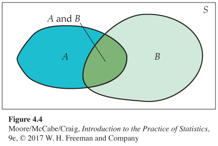
The events A and B are not disjoint. They occur together whenever both tosses give heads. We want to compute the probability of the event {A and B} that both tosses are heads. The Venn diagram in Figure 4.4 illustrates the event {A and B} as the overlapping area that is common to both A and B.
The coin tossing of Buffon, Pearson, and Kerrich described in Example 4.3 makes us willing to assign probability 1/2 to a head when we toss a coin. So
P(A) = 0.5
P(B) = 0.5
What is P(A and B)? Our common sense says that it is 1/4. The first toss will give a head half the time and the second toss will give a head half the time, so both tosses will give heads on 1/2 ×1/2 = 1/4 of all trials in the long run. This reasoning assumes that the second toss still has probability 1/2 of a head after the first has given a head. This is true—we can verify it by tossing a coin twice many times and observing the proportion of heads on the second toss after the first toss has produced a head. We say that the events “head on the first toss” and “head on the second toss” are independent. Here is our final probability rule.
MULTIPLICATION RULE FOR INDEPENDENT EVENTS
Rule 5. Two events A and B are independent if knowing that one occurs does not change the probability that the other occurs. If A and B are independent,
P(A and B) = P(A) P(B)
This is the multiplication rule for independent events.
Our definition of independence is rather informal. We will make this informal idea precise in Section 4.5. In practice, though, we rarely need a precise definition of independence because independence is usually assumed as part of a probability model when we want to describe random phenomena that seem to be physically unrelated to each other. Here is an example of independence.
EXAMPLE 4.16
Coins do not have memory. Because a coin has no memory, we assume that coin tosses are independent. For a fair coin, this means that the outcome of the first toss does not influence the outcome of any other toss.
USE YOUR KNOWLEDGE
Question 4.15
4.15 A head and then a tail in two tosses. What is the probability of obtaining a head and then a tail on two tosses of a fair coin?
4.15 0.25.
Here is an example of a situation where there are dependent events.
EXAMPLE 4.17
Dependent events in cards. The colors of successive cards dealt from the same deck are not independent. A standard 52-card deck contains 26 red and 26 black cards. For the first card dealt from a shuffled deck, the probability of a red card is 26/52 = 0.50 because the 52 possible cards are equally likely. Once we see that the first card is red, we know that there are only 25 reds among the remaining 51 cards. The probability that the second card is red is therefore only 25/51 = 0.49. Knowing the outcome of the first deal changes the probabilities for the second.
USE YOUR KNOWLEDGE
Question 4.16
4.16 The probability of a second ace. A deck of 52 cards contains four aces, so the probability that a card drawn from this deck is an ace is 4/52. If we know that the first card drawn is an ace, what is the probability that the second card drawn is also an ace? Using the idea of independence, explain why this probability is not 4/52.
Here is another example of a situation where events are dependent.
EXAMPLE 4.18
Taking a test twice. If you take an IQ test or other mental test twice in succession, the two test scores are not independent. The learning that occurs on the first attempt influences your second attempt. If you learn a lot, then your second test score might be a lot higher than your first test score.
When independence is part of a probability model, the multiplication rule applies. Here is an example.
EXAMPLE 4.19
Mendel’s peas. Gregor Mendel used garden peas in some of the experiments that revealed that inheritance operates randomly. The seed color of Mendel’s peas can be either green or yellow. Two parent plants are “crossed” (one pollinates the other) to produce seeds.
Each parent plant carries two genes for seed color, and each of these genes has probability 0.5 of being passed to a seed. The two genes that the seed receives, one from each parent, determine its color. The parents contribute their genes independently of each other.
Suppose that both parents carry the G and the Y genes. The seed will be green if both parents contribute a G gene; otherwise, it will be yellow. If M is the event that the male contributes a G gene and F is the event that the female contributes a G gene, then the probability of a green seed is
P(MandF)=P(M)P(F)=(0.5)(0.5)=0.25
In the long run, 1/4 of all seeds produced by crossing these plants will be green.
![]()
The multiplication rule applies only to independent events; you cannot use it if events are not independent. Here is a distressing example of misuse of the multiplication rule.
EXAMPLE 4.20
Sudden infant death syndrome. Sudden infant death syndrome (SIDS) causes babies to die suddenly (often in their cribs) with no explanation. Deaths from SIDS have been greatly reduced by placing babies on their backs, but as yet no cause is known.
When more than one SIDS death occurs in a family, the parents are sometimes accused. One “expert witness” popular with prosecutors in England told juries that there is only a 1 in 73 million chance that two children in the same family could have died from SIDS. Here’s his calculation: the rate of SIDS in a nonsmoking middle-class family is 1 in 8500. So the probability of two deaths is
18500×18500=172,250,000
Several women were convicted of murder on this basis, without any direct evidence that they harmed their children.
As the Royal Statistical Society said, this reasoning is nonsense. It assumes that SIDS deaths in the same family are independent events. The cause of SIDS is unknown: “There may well be unknown genetic or environmental factors that predispose families to SIDS, so that a second case within the family becomes much more likely.”4 The British government decided to review the cases of 258 parents convicted of murdering their babies.
The multiplication rule P(A and B) = P(A)P(B) holds if A and B are independent but not otherwise. The addition rule P(A or B) = P(A) + P(B) holds if A and B are disjoint but not otherwise. Resist the temptation to use these simple formulas when the circumstances that justify them are not present. You must also be certain not to confuse disjointness and independence. Disjoint events cannot be independent. If A and B are disjoint, then the fact that A occurs tells us that B cannot occur—look again at Figure 4.2 (page 224). Unlike disjointness or complements, independence cannot be pictured by a Venn diagram because it involves the probabilities of the events rather than just the outcomes that make up the events. However, it could be displayed in a mosaic plot.
![]()
mosaic plot, p. 143
Applying the probability rules
If two events A and B are independent, then their complements Ac and Bc are also independent and Ac is independent of Bc. Suppose, for example, that 75% of all registered voters in a suburban district are Republicans. If an opinion poll interviews two voters chosen independently, the probability that the first is a Republican and the second is not a Republican is (0.75)(0.25) = 0.1875.
The multiplication rule also extends to collections of more than two events, provided that all are independent. Independence of events A, B, and C means that no information about any one or any two can change the probability of the remaining events. The formal definition is a bit messy. Fortunately, independence is usually assumed in setting up a probability model. We can then use the multiplication rule freely.
By combining the rules we have learned, we can compute probabilities for rather complex events. Here is an example.
EXAMPLE 4.21
HIV testing. Many people who come to clinics to be tested for HIV, the virus that causes AIDS, don’t come back to learn the test results. Clinics now use “rapid HIV tests” that give a result in a few minutes. The false-positive rate for a diagnostic test is the probability that a person with no disease will have a positive test result. For the rapid HIV tests, the Food and Drug Administration (FDA) has established 2% as the maximum false-positive rate allowed.5 If a clinic uses a test that matches the FDA standard and tests 50 people who are free of HIV antibodies, what is the probability that at least one false-positive will occur?
It is reasonable to assume as part of the probability model that the test results for different individuals are independent. The probability that the test is positive for a single person is 0.02, so the probability of a negative result is 1 − 0.02 = 0.98 by the complement rule. The probability of at least one false-positive among the 50 people tested is, therefore,
P(at least 1 positive)=1-P(no positives)=1-P(50 negatives)=1-0.9850=1-0.3642=0.6358
There is approximately a 64% chance that at least 1 of the 50 people will test positive for HIV even though none of them has the virus.
Concern about excessive numbers of false-positives led the New York City Department of Health and Mental Hygiene to suspend the use of one particular rapid HIV test.6