5.2 5.2 The Sampling Distribution of a Sample Mean
When you complete this section, you will be able to:
• Explain the difference between the sampling distribution of ˉx and the population distribution.
• Determine the mean and standard deviation of ˉx for an SRS of size n from a population with mean μ and standard deviation σ.
• Describe how much larger n has to be for an SRS to reduce the standard deviation of ˉx by a certain factor.
• Utilize the central limit theorem to approximate the sampling distribution of ˉx and perform probability calculations based on this approximation.
A variety of statistics are used to describe quantitative data. The sample mean, median, and standard deviation are all examples of statistics based on quantitative data. Statistical theory describes the sampling distributions of these statistics. However, the general framework for constructing a sampling distribution is the same for all statistics. In this section, we will concentrate on the sample mean. Because sample means are just averages of observations, they are among the most frequently used statistics.
Suppose that you plan to survey 1000 undergraduates enrolled in four-year U.S. universities about their sleeping habits. The sampling distribution of the average hours of sleep per night describes what this average would be if many simple random samples of 1000 students were drawn from the population of students in the United States. In other words, it gives you an idea of what you are likely to see from your survey. It tells you whether you should expect this average to be near the population mean and whether the variation of the statistic is roughly ±2 hours or ±2 minutes.
Before constructing this distribution, however, we need to consider another set of probability distributions that also plays a role in statistical inference. Any quantity that can be measured on each member of a population is described by the distribution of its values for all members of the population. This is the context in which we first met distributions, as density curves that provide models for the overall pattern of data.
density curves, p. 51
Imagine choosing one individual at random from a population and measuring a quantity. The quantities obtained from repeated draws of one individual from a population have a probability distribution that is the distribution of the population.
EXAMPLE 5.4
Total sleep time of college students. A recent survey describes the distribution of total sleep time among college students as approximately Normal with a mean of 6.78 hours and standard deviation of 1.24 hours.3 Suppose that we select a college student at random and obtain his or her sleep time. This result is a random variable X because, prior to the random sampling, we don’t know the sleep time. We do know, however, that in repeated sampling, X will have the same N(6.78, 1.24) distribution that describes the pattern of sleep time in the entire population. We call N(6.78, 1.24) the population distribution.
POPULATION DISTRIBUTION
The population distribution of a variable is the distribution of its values for all members of the population. The population distribution is also the probability distribution of the variable when we choose one individual at random from the population.
In this example, the population of all college students actually exists so that we can, in principle, draw an SRS of students from it. Sometimes, our population of interest does not actually exist. For example, suppose that we are interested in studying final-exam scores in a statistics course, and we have the scores of the 34 students who took the course last semester. For the purposes of statistical inference, we might want to consider these 34 students as part of a hypothetical population of similar students who would take this course. In this sense, these 34 students represent not only themselves, but also a larger population of similar students. The key idea is to think of the observations that you have as coming from a population with a probability distribution.
USE YOUR KNOWLEDGE
Question 5.17
5.17 Time spent using apps on a mobile device. Nielsen has installed, with permission, Mobile Netview 3 on approximately 5000 cell phones to gather information on mobile app usage among adults in the United States. Nielsen reported that 18–24 year olds spend an average of 37 hours and 6 minutes a month using mobile apps.4 State the population that this survey describes, the statistic, and some likely values from the population distribution.
5.17 Population: all adults in the United States. Statistic: mean of 37 hours and 6 minutes. Likely values: answers will vary, any amount of time someone could spend during a month using mobile apps.
Now that we have made the distinction between the population distributions and sampling distributions, we can proceed with an in-depth study of the sampling distribution of a sample mean ˉx.
EXAMPLE 5.5
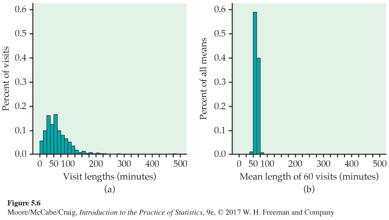
Sample means are approximately Normal. Figure 5.6 illustrates two striking facts about the sampling distribution of a sample mean. Figure 5.6(a) displays the distribution of student visit lengths (in minutes) to a statistics help room at a large midwestern university. Students visiting the help room were asked to sign in upon arrival and then sign out when leaving. During the school year, there were 1838 visits to the help room but only 1264 recorded visit lengths. This is because many visiting students forgot to sign out. We also omitted a few large outliers (visits lasting more than 10 hours).5 The distribution is strongly skewed to the right. The population mean is μ = 61.28 minutes.
| 10 | 14 | 15 | 16 | 18 | 20 | 20 | 20 | 23 | 25 |
| 28 | 30 | 30 | 30 | 30 | 30 | 31 | 33 | 35 | 35 |
| 46 | 48 | 50 | 50 | 50 | 50 | 51 | 54 | 55 | 55 |
| 60 | 60 | 60 | 60 | 60 | 60 | 60 | 65 | 65 | 65 |
| 75 | 77 | 80 | 80 | 84 | 85 | 88 | 98 | 100 | 100 |
| 105 | 105 | 105 | 115 | 120 | 135 | 135 | 136 | 157 | 210 |
Table 5.1 contains the lengths of a random sample of 60 visits from this population. The mean of these 60 visits is ˉx = 63.45 minutes. If we were to take another sample of size 60, we would likely get a different value of ˉx. This is because this new sample would contain a different set of visits. To find the sampling distribution of ˉx, we take many SRSs of size 60 and calculate ˉx for each sample. Figure 5.6(b) is the distribution of the values of ˉx for 500 random samples. The scales and choice of classes are exactly the same as in Figure 5.6(a) so that we can make a direct comparison.
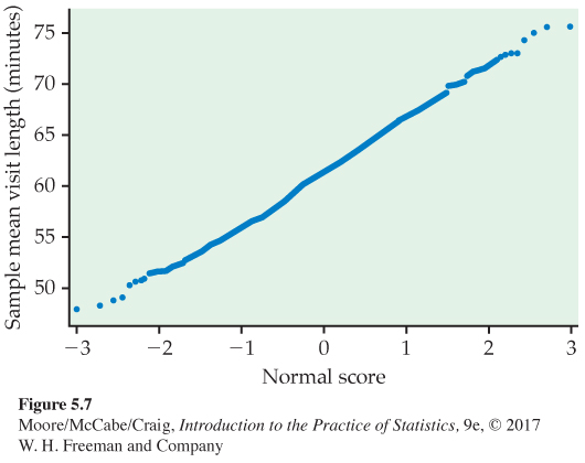
The sample means are much less spread out than the individual visit lengths. What is more, the Normal quantile plot in Figure 5.7 confirms that the distribution in Figure 5.6(b) is close to Normal.
This example illustrates two important facts about sample means that we will discuss in this section.
FACTS ABOUT SAMPLE MEANS
1. Sample means are less variable than individual observations.
2. Sample means are more Normal than individual observations.
These two facts contribute to the popularity of sample means in statistical inference.
The mean and standard deviation of ˉx
The sample mean ˉx from a sample or an experiment is an estimate of the mean μ of the underlying population. The sampling distribution of ˉx is determined by
• the design used to produce the data,
• the sample size n, and
• the population distribution.
Select an SRS of size n from a population, and measure a variable X on each individual in the sample. The n measurements are values of n random variables X1, X2, . . . , Xn. A single Xi is a measurement on one individual selected at random from the population and, therefore, has the distribution of the population. If the population is large relative to the sample, we can consider X1, X2 , . . . , Xn to be independent random variables, each having the same distribution. This is our probability model for measurements on each individual in an SRS.
The sample mean of an SRS of size n is
ˉx=1n(X1+X2+⋯Xn)
rules for means, p. 254
If the population has mean μ, then μ is the mean of the distribution of each observation Xi. To get the mean of ˉx, we use the rules for means of random variables. Specifically,
μˉx=1n(μX1+μX2+⋯+μXn)=1n(μ+μ+⋯+μ)=μ
rules for variances, p. 258
That is, the mean of ˉx is the same as the mean of the population. The sample mean ˉx is, therefore, an unbiased estimator of the unknown population mean μ.
The observations are independent, so the addition rule for variances also applies:
σ2ˉx=(1n)2(σ2X1+σ2X2+⋯+σ2Xn)=(1n)2(σ2+σ2+⋯+σ2)=σ2n
With n in the denominator, the variability of ˉx about its mean decreases as the sample size grows. Thus, a sample mean from a large sample will usually be very close to the true population mean μ. Here is a summary of these facts.
MEAN AND STANDARD DEVIATION OF A SAMPLE MEAN
Let ˉx be the mean of an SRS of size n from a population having mean μ and standard deviation σ. The mean and standard deviation of ˉx are
μ¯x=μσˉx=σ√n
How precisely does a sample mean ˉx estimate a population mean μ? Because the values of ˉx vary from sample to sample, we must give an answer in terms of the sampling distribution. We know that ˉx is an unbiased estimator of μ, so its values in repeated samples are not systematically too high or too low. Most samples will give an ˉx-value close to μ if the sampling distribution is concentrated close to its mean μ. So the precision of estimation depends on the spread of the sampling distribution.
Because the standard deviation of ˉx is σ/√n, the standard deviation of the statistic decreases in proportion to the square root of the sample size. This means, for example, that a sample size must be multiplied by 4 in order to divide the statistic’s standard deviation in half. By comparison, a sample size must be multiplied by 100 in order to reduce the standard deviation by a factor of 10.
EXAMPLE 5.6
Standard deviations for sample means of visit lengths. The standard deviation of the population of visit lengths in Figure 5.6(a) is σ = 41.84 minutes. The length of a single visit will often be far from the population mean. If we choose an SRS of 15 visits, the standard deviation of their mean length is
σˉx=41.84√15=10.80 minutes
Averaging over more visits reduces the variability and makes it more likely that ˉx is close to μ. Our sample size of 60 visits is 4 times 15, so the standard deviation will be half as large:
σˉx=41.84√60=5.40 minutes
USE YOUR KNOWLEDGE
Question 5.18
5.18 Find the mean and the standard deviation of the sampling distribution. Compute the mean and standard deviation of the sampling distribution of the sample mean when you plan to take an SRS of size 64 from a population with mean 44 and standard deviation 16.
Question 5.19
5.19 The effect of increasing the sample size. In the setting of the previous exercise, repeat the calculations for a sample size of 576. Explain the effect of the sample size increase on the mean and standard deviation of the sampling distribution.
5.19 μˉx=44. σˉx=0.667.
The central limit theorem
We have described the center and spread of the probability distribution of a sample mean ˉx, but not its shape. The shape of the distribution of ˉx depends on the shape of the population distribution. Here is one important case: if the population distribution is Normal, then so is the distribution of the sample mean.
SAMPLING DISTRIBUTION OF A SAMPLE MEAN
If a population has the N(μ, σ) distribution, then the sample mean ˉx of n independent observations has the N(μ, σ/√n) distribution.
This is a somewhat special result. Many population distributions are not Normal. The help room visit lengths in Figure 5.6(a), for example, are strongly skewed. Yet Figure 5.6(b) and 5.7 show that means of samples of size 60 are close to Normal.
One of the most famous facts of probability theory says that, for large sample sizes, the distribution of ˉx is close to a Normal distribution. This is true no matter what shape the population distribution has, as long as the population has a finite standard deviation σ. This is the central limit theoremcentral limit theorem. It is much more useful than the fact that the distribution of ˉx is exactly Normal if the population is exactly Normal.
CENTRAL LIMIT THEOREM
Draw an SRS of size n from any population with mean μ and finite standard deviation σ. When n is large, the sampling distribution of the sample mean ˉx is approximately Normal:
ˉx is approximately N(μ, σ√n)
EXAMPLE 5.7
How close will the sample mean be to the population mean? With the Normal distribution to work with, we can better describe how precisely a random sample of 60 visits estimates the mean length of all visits to the help room. The population standard deviation for the 1264 visits in the population of Figure 5.6(a) is σ = 41.84 minutes. From Example 5.6 we know σˉx=5.4 minutes. By the 95 part of the 68–95–99.7 rule, about 95% of all samples will have mean ˉx within two standard deviations of μ, that is, within ±10.8 minutes of μ.
68–95–99.7 rule, p. 57
USE YOUR KNOWLEDGE
Question 5.20
5.20 Use the 68–95–99.7 rule. You take an SRS of size 64 from a population with mean 82 and standard deviation 24. According to the central limit theorem, what is the approximate sampling distribution of the sample mean? Use the 95 part of the 68–95–99.7 rule to describe the variability of ˉx.
For the sample size of n = 60 in Example 5.7, the sample mean is not very precise. The population of help room visit lengths is very spread out, so the sampling distribution of ˉx has a large standard deviation.
EXAMPLE 5.8
How can we reduce the standard deviation? In the setting of Example 5.7, if we want to reduce the standard deviation of ˉx by a factor of 2, we must take a sample four times as large, n = 4 × 60, or 240. Then
σˉx=41.84√240=2.70 minutes
For samples of size 240, about 95% of the sample means will be within twice 2.70, or 5.40 minutes, of the population mean μ.
![]()
The standard deviation computed in Example 5.8 is actually too large. This is due to the fact that the population size, N = 1264, is not at least 20 times larger than the sample size, n = 240. In these settings, it is better to adjust the standard deviation of ˉx to reflect only the variance remaining in the population that is not in the sample. This is done by multiplying the unadjusted standard deviation by the finite population correction factorfinite population
correction factor. This quantity is √N−nN−1 and moves the standard deviation of ˉx toward 0 as n moves toward N. Applying this correction to Example 5.8, the standard deviation of ˉx is reduced 10% to
41.84√240√1264−2401264−1=2.43 minutes
Thus, for samples of size 240, about 95% of the sample means will be within twice 2.43, or 4.86 minutes, of the population mean μ, rather than the 5.40 minutes reported in Example 5.8.
USE YOUR KNOWLEDGE
Question 5.21
5.21 The effect of increasing the sample size. In the setting of Exercise 5.20, suppose that we increase the sample size to 2304. Use the 95 part of the 68–95–99.7 rule to describe the variability of this sample mean. Compare your results with those you found in Exercise 5.20.
5.21 About 95% of the time, ˉx should be between 81 and 83.
Example 5.8 reminds us that if the population is very spread out, the √n in the formula for the deviation of ˉx implies that very large samples are needed to estimate the population mean precisely. The main point of the example, however, is that the central limit theorem allows us to use Normal probability calculations to answer questions about sample means even when the population distribution is not Normal.
How large a sample size n is needed for ˉx to be close to Normal depends on the population distribution. More observations are required if the shape of the population distribution is far from Normal. For the very skewed visit length population, samples of size 60 are large enough. Further study would be needed to see if the distribution of ˉx is close to Normal for smaller samples like n = 20 or n = 40. Here is a more detailed study of another skewed distribution.
EXAMPLE 5.9
The central limit theorem in action. Figure 5.8 shows the central limit theorem in action for another very non-Normal population. Figure 5.8(a) displays the density curve of a single observation from the population. The distribution is strongly right-skewed, and the most probable outcomes are near 0. The mean μ of this distribution is 1, and its standard deviation σ is also 1. This particular continuous distribution is called an exponential distributionexponential distribution. Exponential distributions are used as models for how long an iPhone will function properly and for the time between snaps you receive on Snapchat.
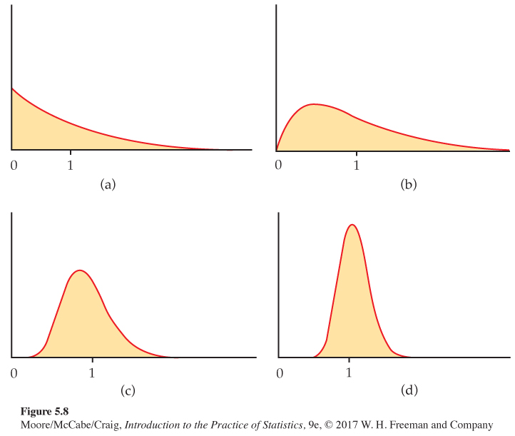
Figure 5.8(b), (c), and (d) are the density curves of the sample means of 2, 10, and 25 observations from this population. As n increases, the shape becomes more Normal. The mean remains at μ = 1, but the standard deviation decreases, taking the value 1/√n. The density curve for 10 observations is still somewhat skewed to the right but already resembles a Normal curve having μ = 1 and σ=1/√10=0.32. The density curve for n = 25 is yet more Normal. The contrast between the shape of the population distribution and of the distribution of the mean of 10 or 25 observations is striking.
You can also use the Central Limit Theorem applet to study the sampling distribution of ˉx. From one of three population distributions, 10,000 SRSs of a user-specified sample size n are generated, and a histogram of the sample means is constructed. You can then compare this estimated sampling distribution with the Normal curve that is based on the central limit theorem.
EXAMPLE 5.10
Using the Central Limit Theorem applet. In Example 5.9, we considered sample sizes of n = 2, 10, and 25 from an exponential distribution. Figure 5.9 shows a screenshot of the Central Limit Theorem applet for the exponential distribution when n = 10. The mean and standard deviation of this sampling distribution are 1 and 1/√10=0.316, respectively. From the 10,000 SRSs, the mean is estimated to be 1.001 and the estimated standard deviation is 0.319. These are both quite close to the true values. In Figure 5.8(c), we saw that the density curve for 10 observations is still somewhat skewed to the right. We can see this same behavior in Figure 5.9 when we compare the histogram with the Normal curve based on the central limit theorem.
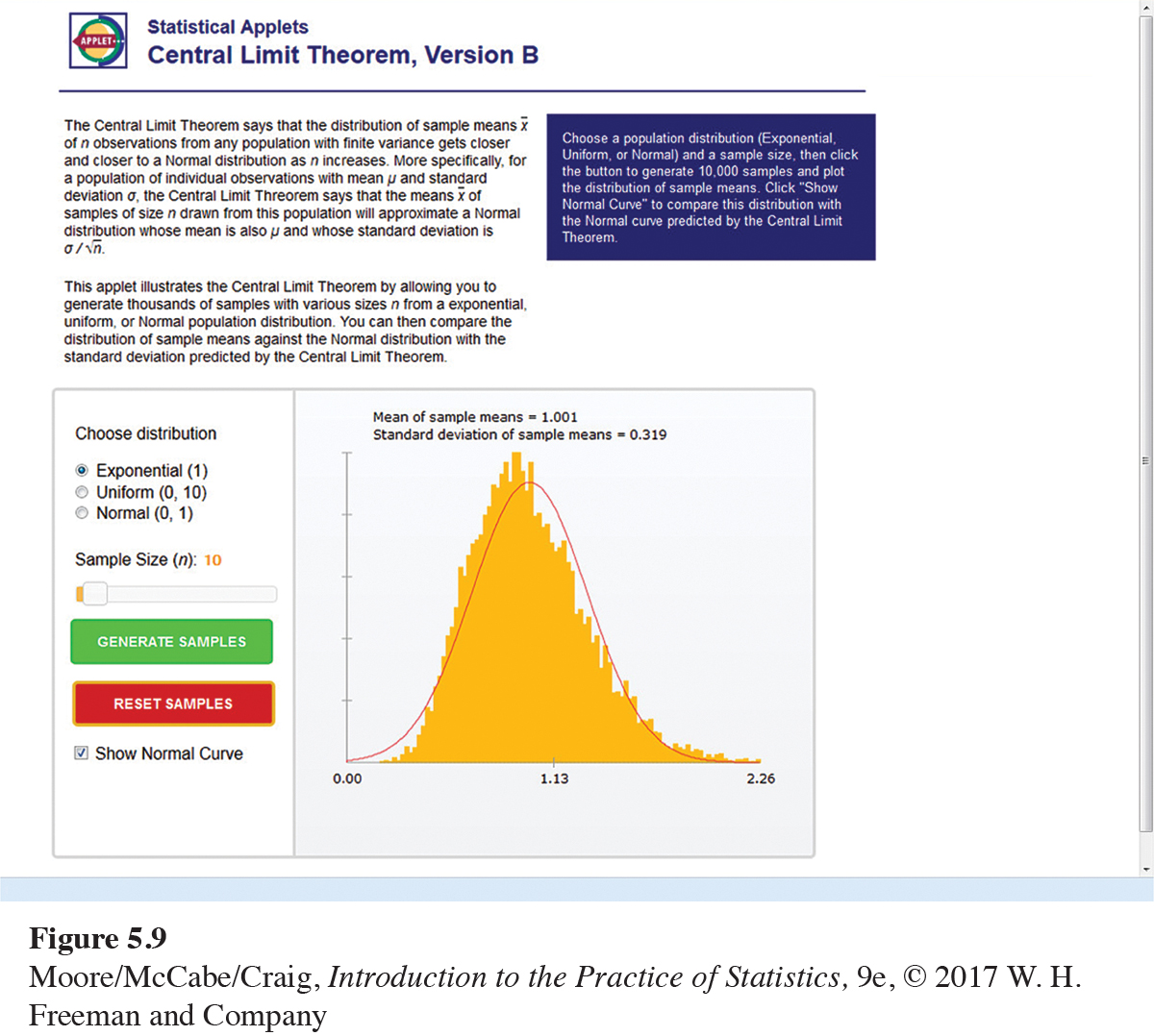
Try using the applet for the other sample sizes in Example 5.9. You should get histograms shaped like the density curves shown in Figure 5.8. You can also consider other sample sizes by sliding n from 1 to 100. As you increase n, the shape of the histogram moves closer to the Normal curve that is based on the central limit theorem.
USE YOUR KNOWLEDGE
Question 5.22
5.22 Use the Central Limit Theorem applet. Let’s consider the uniform distribution between 0 and 10. For this distribution, all intervals of the same length between 0 and 10 are equally likely. This distribution has a mean of 5 and standard deviation of 2.89.
- Page 302
(a) Approximate the population distribution by setting n = 1 and clicking the “Generate samples” button.
(b) What are your estimates of the population mean and population standard deviation based on the 10,000 SRSs? Are these population estimates close to the true values?
(c) Describe the shape of the histogram and compare it with the Normal curve.
Question 5.23
5.23 Use the Central Limit Theorem applet again. Refer to the previous exercise. In the setting of Example 5.9, let’s approximate the sampling distribution for samples of size n = 2, 10, and 25 observations.
(a) For each sample size, compute the mean and standard deviation of ˉx.
(b) For each sample size, use the applet to approximate the sampling distribution. Report the estimated mean and standard deviation. Are they close to the true values calculated in part (a)?
(c) For each sample size, compare the shape of the sampling distribution with the Normal curve based on the central limit theorem.
(d) For this population distribution, what sample size do you think is needed to make you feel comfortable using the central limit theorem to approximate the sampling distribution of ˉx? Explain your answer.
5.23 (a) Each sample size has μˉx=1. For n = 2, σˉx=0.7071. For n = 10, σˉx=0.3162. For n = 25, σˉx=0.2.
Now that we know that the sampling distribution of the sample mean ˉx is approximately Normal for a sufficiently large n, let’s consider some probability calculations.
EXAMPLE 5.11
Time between snaps. Snapchat has more than 100 million daily users sending well over 400 million snaps a day.6 Suppose that the time X between snaps received is governed by the exponential distribution with mean μ = 15 minutes and standard deviation σ = 15 minutes. You record the next 50 times between snaps. What is the probability that their average exceeds 13 minutes?
The central limit theorem says that the sample mean time ˉx (in minutes) between snaps has approximately the Normal distribution with mean equal to the population mean μ = 15 minutes and standard deviation
σ√50=15√50=2.12 minutes
The sampling distribution of ˉx is, therefore, approximately N(15,2.12). Figure 5.10 shows this Normal curve (solid) and also the actual density curve of ˉx (dashed).
The probability we want is P(ˉx>13.0). This is the area to the right of 13 under the solid Normal curve in Figure 5.10. A Normal distribution calculation gives
P(ˉx>13.0)=P(ˉx−152.12>13.0−152.12)
= P (Z > −0.94) = 0.8264
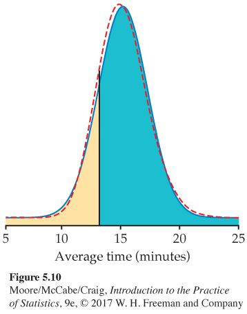
The exactly correct probability is the area under the dashed density curve in the figure. It is 0.8265. The central limit theorem Normal approximation is off by only about 0.0001.
We can also use this sampling distribution to talk about the total time between the 1st and 51st snap received.
EXAMPLE 5.12
Convert the results to the total time. There are 50 time intervals between the 1st and 51st snap. According to the central limit theorem calculations in Example 5.11,
P(ˉx>13.0)=0.8264
We know that the sample mean is the total time divided by 50, so the event {ˉx>13.0} is the same as the event {50ˉx>50(13.0)}. We can say that the probability is 0.8264 that the total time is 50(13.0) = 650 minutes (10.8 hours) or greater.
USE YOUR KNOWLEDGE
Question 5.24
5.24 Find a probability. Refer to Example 5.11. Find the probability that the mean time between snaps is less than 15 minutes. The exact probability is 0.5188. Compare your answer with the exact one.
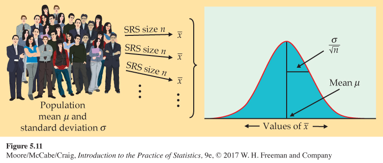
Figure 5.11 summarizes the facts about the sampling distribution of ˉx in a way that emphasizes the big idea of a sampling distribution. The general framework for constructing the sampling distribution of ˉx is shown on the left.
• Take many random samples of size n from a population with mean μ and standard deviation σ.
• Find the sample mean ˉx for each sample.
• Collect all the ˉx’s and display their distribution.
The sampling distribution of ˉx is shown on the right. Keep this figure in mind as you go forward.
A few more facts
The central limit theorem is the big fact of probability theory in this section. Here are three additional facts related to our investigations that will be useful in describing methods of inference in later chapters.
The fact that the sample mean of an SRS from a Normal population has a Normal distribution is a special case of a more general fact: any linear combination of independent Normal random variables is also Normally distributed. That is, if X and Y are independent Normal random variables and a and b are any fixed numbers, aX + bY is also Normally distributed, and this is true for any number of Normal random variables. In particular, the sum or difference of independent Normal random variables has a Normal distribution. The mean and standard deviation of aX + bY are found as usual from the rules for means and variances. These facts are often used in statistical calculations. Here is an example.
EXAMPLE 5.13
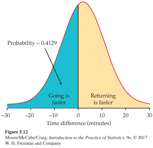
Getting to and from campus. You live off campus and take the shuttle, provided by your apartment complex, to and from campus. Your time on the shuttle in minutes varies from day to day. The time going to campus X has the N(20,4) distribution, and the time returning from campus Y varies according to the N(18, 8) distribution. If they vary independently, what is the probability that you will be on the shuttle for less time going to campus?
The difference in times X − Y is Normally distributed, with mean and variance
μX−Y = μX − μY = 20 − 18 = 2
σ2X−Y=σ2X+σ2Y=42+82=80
Because √80=8.94, X − Y has the N(2, 8.94) distribution. Figure 5.12 illustrates the probability computation:
P(X < Y) = P(X − Y < 0)
=P((X−Y)−28.94 < 0−28.94)
= P(Z < −0.22) = 0.4129
Although, on average, it takes longer to go to campus than return, the trip to campus will take less time on roughly two of every five days.
The second useful fact is that more general versions of the central limit theorem say that the distribution of a sum or average of many small random quantities is close to Normal. This is true even if the quantities are not independent (as long as they are not too highly correlated) and even if they have different distributions (as long as no single random quantity is so large that it dominates the others). These more general versions of the central limit theorem suggest why the Normal distributions are common models for observed data. Any variable that is a sum of many small random influences will have approximately a Normal distribution.
Finally, the central limit theorem also applies to discrete random variables. An average of discrete random variables will never result in a continuous sampling distribution, but the Normal distribution often serves as a good approximation. In Section 5.3, we will discuss the sampling distribution and Normal approximation for counts and proportions. This Normal approximation is just an example of the central limit theorem applied to these discrete random variables.
BEYOND THE BASICS
Weibull Distributions
Our discussion of sampling distributions so far has concentrated on the Normal model to approximate the sampling distribution of the sample mean ˉx. This model is important in statistical practice because of the central limit theorem and the fact that sample means are among the most frequently used statistics. Simplicity also contributes to its popularity. The parameter μ is easy to understand, and to estimate it, we use a statistic ˉx that is also easy to understand and compute.
There are, however, many other probability distributions that are used to model data in various circumstances. The time that a product, such as a computer hard drive, lasts before failing rarely has a Normal distribution. Earlier, we mentioned the use of the exponential distribution to model time to failure. Another class of continuous distributions, the Weibull distributionsWeibull distributions, is more commonly used in these situations.
EXAMPLE 5.14
Weibull density curves. Figure 5.13 shows the density curves of three members of the Weibull family. Each describes a different type of distribution for the time to failure of a product.
1. The top curve in Figure 5.13 is a model for infant mortality. This describes products that often fail immediately, prior to delivery to the customer. However, if the product does not fail right away, it will likely last a long time. For products like this, a manufacturer might test them and ship only the ones that do not fail immediately.
2. The middle curve in Figure 5.13 is a model for early failure. These products do not fail immediately, but many fail early in their lives after they are in the hands of customers. This is disastrous—the product or the process that makes it must be changed at once.
3. The bottom curve in Figure 5.13 is a model for old-age wear-out. Most of these products fail only when they begin to wear out, and then many fail at about the same age.
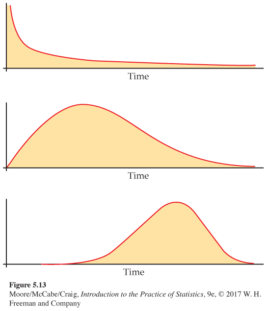
A manufacturer certainly wants to know to which of these classes a new product belongs. To find out, engineers operate a random sample of products until they fail. From the failure time data, we can estimate the parameter (called the “shape parameter”) that distinguishes among the three Weibull distributions in Figure 5.13. The shape parameter has no simple definition like that of a population proportion or mean, and it cannot be estimated by a simple statistic such as ˆp or ˉx.
Two things save the situation. First, statistical theory provides general approaches for finding good estimates of any parameter. These general methods not only tell us how to use ˉx in the Normal settings, but also how to estimate the Weibull shape parameter. Second, software can calculate the estimate from data even though there is no algebraic formula that we can write for the estimate. Statistical practice often relies on both mathematical theory and methods of computation more elaborate than the ones we will meet in this book. Fortunately, big ideas such as sampling distributions carry over to more complicated situations.7