All economic decisions are about comparing costs and benefits—and usually about comparing marginal costs and marginal benefits. This goes both for a consumer, deciding whether to buy more goods or services, and for a firm, deciding whether to hire an additional worker.

Although there are some important exceptions, most factor markets in the modern American economy are perfectly competitive. This means that most buyers and sellers of factors are price-takers because they are too small relative to the market to do anything but accept the market price. And in a competitive labor market, it’s clear how to define the marginal cost an employer pays for a worker: it is simply the worker’s wage rate. But what is the marginal benefit of that worker? To answer that question, we return to the production function, which relates inputs to output. We begin by examining a firm that is a price-taker in the output market—that is, it operates in a perfectly competitive industry.

691

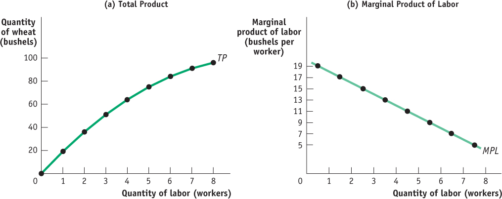
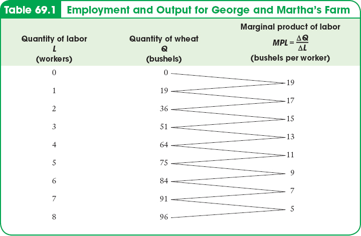
Figure 69.2 shows the production function for wheat on George and Martha’s farm, as introduced in Module 54. Panel (a) uses the total product curve to show how total wheat production depends on the number of workers employed on the farm; panel (b) shows how the marginal product of labor, the increase in output from employing one more worker, depends on the number of workers employed. Table 69.1 shows the numbers behind the figure. Note: sometimes the marginal product (MP) is called the marginal physical product or MPP. These two terms are the same; the extra “P” just emphasizes that the term refers to the quantity of physical output being produced, not the monetary value of that output.

If workers are paid $200 each and George and Martha can sell an unlimited amount of wheat for $20 per bushel, how many workers should George and Martha employ to maximize profit?

Earlier we showed how to answer this question in several steps. First, we used information from the production function to derive the firm’s total cost and its marginal cost. Then we used the price-taking firm’s optimal output rule: a price-taking firm’s profit is maximized by producing the quantity of output at which the marginal cost is equal to the market price. Having determined the optimal quantity of output, we went back to the production function to find the optimal number of workers—which was simply the number of workers needed to produce the optimal quantity of output.

As you might have guessed, marginal analysis provides a more direct way to find the number of workers that maximizes a firm’s profit. This alternative approach is just a different way of looking at the same thing. But it gives us more insight into the demand for factors as opposed to the supply of goods.

692

To see how this alternative approach works, suppose that George and Martha are deciding whether to employ another worker. The increase in cost from employing another worker is the wage rate, W, at which the firm can hire any number of workers in a perfectly competitive labor market. The benefit to George and Martha from employing another worker is the additional revenue gained from the hire. To determine the change in revenue, we can multiply the marginal product of labor, MPL, by the marginal revenue received from selling the additional output, MR. This amount—the additional revenue generated by employing one more unit of labor—is known as the marginal revenue product of labor, or MRPL:

(69-1) Marginal revenue product of labor = MRPL = MPL × MR

So should George and Martha hire another worker? Yes, if the resulting increase in revenue exceeds the cost of the additional worker—that is, if MRPL > W. Otherwise, they should not.

The hiring decision is made using marginal analysis, by comparing the marginal benefit from hiring another worker (MRPL) with the marginal cost (W). And as with any decision that is made on the margin, the optimal choice is made by equating marginal benefit with marginal cost (or if they’re never equal, by continuing to hire until the marginal cost of one more unit would exceed the marginal benefit). So to maximize profit, George and Martha will employ workers up to the point at which, for the last worker employed,

(69-2) MRPL = W.

This rule isn’t limited to labor; it applies to any factor of production. The marginal revenue product of any factor is its marginal product times the marginal revenue received from the good it produces. And as a general rule, profit-maximizing, price-taking firms will keep adding more units of each factor of production until the marginal revenue product of the last unit employed is equal to the factor’s price.

This rule is consistent with our previous analysis. We saw that a profit-maximizing firm chooses the level of output at which the marginal revenue of the good it produces equals the marginal cost of producing that good. It turns out that if the level of output is chosen so that marginal revenue equals marginal cost, then it is also true that with the amount of labor required to produce that output level, the marginal revenue product of labor will equal the wage rate.

693

Now let’s look more closely at why firms should choose the level of employment that equates MRPL and W, and at how that decision helps us understand factor demand.

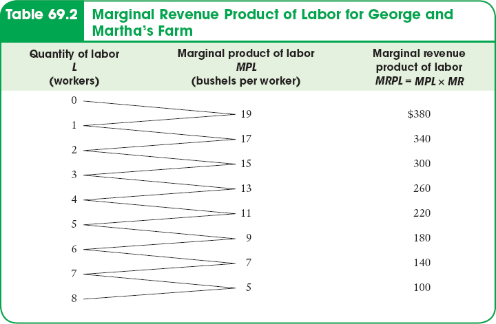
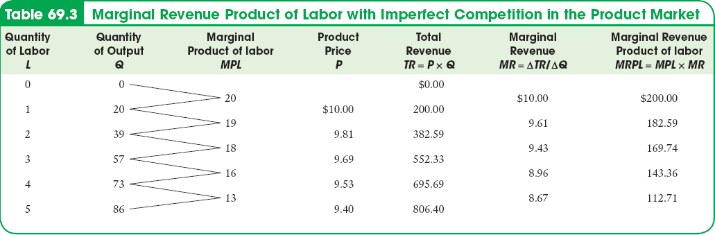
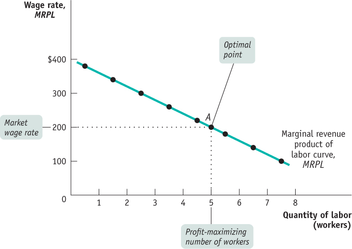
Table 69.2 shows the marginal revenue product of labor on George and Martha’s farm when the price of wheat (and thus the marginal revenue for this price-taking firm) is $20 per bushel. In Figure 69.3, the horizontal axis shows the number of workers employed; the vertical axis measures the marginal revenue product of labor and the wage rate. The curve shown is the marginal revenue product curve of labor. This curve, like the marginal revenue product of labor curve, slopes downward because of diminishing returns to labor in production. That is, the marginal revenue product of each worker is less than that of the preceding worker because the marginal product of each worker is less than that of the preceding worker. For a firm that is not a price-taker, the curve also slopes downward because marginal revenue decreases as more units are sold.

694

We have just seen that to maximize profit, George and Martha hire workers until the wage rate is equal to the marginal revenue product of the last worker employed. Let’s use the example to see how this principle really works.

Assume that George and Martha currently employ 3 workers and that these workers must be paid the market wage rate of $200. Should they employ an additional worker?

Looking at Table 69.2, we see that if George and Martha currently employ 3 workers, the marginal revenue product of an additional worker is $260. So if they employ an additional worker, they will increase their revenue by $260 but increase their cost by only $200, yielding a $60 increase in profit. In fact, a firm can always increase profit by employing one more unit of a factor of production as long as the marginal revenue product of that unit exceeds the factor price.

Alternatively, suppose that George and Martha employ 8 workers. By reducing the number of workers to 7, they can save $200 in wages. In addition, the marginal revenue product of the 8th worker is only $100. So, by reducing employment by one worker, they can increase profit by $200 - $100 = $100. In other words, a firm can always increase profit by employing one less unit of a factor of production as long as the marginal revenue product of that unit is less than the factor price.

Using this method, we can see from Table 69.2 that the profit-maximizing employment level is 5 workers, given a wage rate of $200. The marginal revenue product of the 5th worker is $220, so adding the 5th worker results in $220 of additional revenue ($20 of additional profit). But George and Martha should not hire more than 5 workers: the marginal revenue product of the 6th worker is only $180, $20 less than the cost of that worker. So, to maximize profit, George and Martha should employ workers up to but not beyond the point at which the marginal revenue product of the last worker employed is equal to the wage rate.

Look again at the marginal revenue product curve in Figure 69.3. To determine the profit-maximizing level of employment, we set the marginal revenue product of labor equal to the price of labor—a wage rate of $200 per worker. This means that the profit-maximizing level of employment is at point A, corresponding to an employment level of 5 workers. If the wage rate were higher than $200, we would simply move up the curve and decrease the number of workers employed: if the wage rate were lower than $200, we would move down the curve and increase the number of workers employed.

In this example, George and Martha have a small farm in which the potential employment level varies from 0 to 8 workers, and they hire workers up to the point at which the marginal revenue product of another worker would fall below the wage rate. For a larger farm with many employees, the marginal revenue product of labor falls only slightly when an additional worker is employed. As a result, there will be some worker whose marginal revenue product almost exactly equals the wage rate. (In keeping with the George and Martha example, this means that some worker generates a marginal revenue product of approximately $200.) In this case, the firm maximizes profit by choosing a level of employment at which the marginal revenue product of the last worker hired equals (to a very good approximation) the wage rate.

In the interest of simplicity, we will assume from now on that firms use this rule to determine the profit-maximizing level of employment. This means that the marginal revenue product of labor curve is the individual firm’s labor demand curve. And in general, a firm’s marginal revenue product curve for any factor of production is that firm’s individual demand curve for that factor of production.

695

Because many firms are not price-takers, let’s now consider the marginal revenue product for a firm in an imperfectly competitive market. Suppose John and Abigail own the only pizzeria in their town, and like all monopolists, they must lower their price in order to sell more pizzas. In this case, due to the price effect, the marginal revenue gained from each pizza is less than its price. Table 69.3 shows the calculation of the marginal revenue product for each of John and Abigail’s workers. For example, by hiring the 3rd worker, they are able to produce 18 additional pizzas. The marginal revenue received from these pizzas is $9.69, so the marginal revenue product of the 3rd worker is 18 × $9.69 = $169.74.

As in the case of ordinary demand curves, it is important to distinguish between movements along the factor demand curve and shifts of the factor demand curve. What causes factor demand curves to shift? There are three main causes:

Changes in the Prices of Goods Remember that factor demand is derived demand: if the price of the good that is produced with a factor changes, so will the marginal revenue received from the good and thus the marginal revenue product of the factor. That is, in the case of labor demand, if P changes, MR changes, and MRPL = MPL × MR will change at any given level of employment.

Figure 69.4 illustrates the effects of changes in the price of wheat on George and Martha’s demand for labor, assuming that $200 is the current wage rate. Panel (a) shows the effect of an increase in the price of wheat. Note that the price increase is the same as the marginal revenue increase here because P = MR in a perfectly competitive market. This increase shifts the marginal revenue product of labor curve upward because MRPL rises at any given level of employment. If the wage rate remains unchanged at $200, then the optimal point moves from point A to point B: the profit-maximizing level of employment rises from 5 to 8 workers.

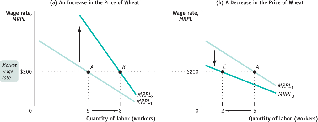
Panel (b) shows the effect of a decrease in the price of wheat. This shifts the marginal revenue product of labor curve downward. If the wage rate remains unchanged at $200, then the optimal point moves from point A to point C: the profit-maximizing level of employment falls from 5 to 2 workers.

696

Changes in the Supply of Other Factors Suppose that George and Martha acquire more land to cultivate—say, by clearing a woodland on their property. Each worker now produces more wheat because each one has more land to work with. As a result, the marginal product of labor on the farm rises at any given level of employment. This has the same effect as an increase in the price of wheat, which is illustrated in panel (a) of Figure 69.4: the marginal revenue product of labor curve shifts upward, and at any given wage rate the profit-maximizing level of employment rises. Similarly, suppose George and Martha cultivate less land. This leads to a fall in the marginal product of labor at any given employment level. Each worker produces less wheat because each has less land to work with. As a result, the marginal revenue product of labor curve shifts downward—as in panel (b) of Figure 69.4—and the profit-maximizing level of employment falls.

Changes in Technology In general, the effect of technological progress on the demand for any given factor can go either way: improved technology can either increase or decrease the demand for a given factor of production.

How can technological progress decrease factor demand? Consider horses, which were once an important factor of production. The development of substitutes for horse power, such as automobiles and tractors, greatly reduced the demand for horses.

The usual effect of technological progress, however, is to increase the demand for a given factor, often because it raises the marginal product of the factor. In particular, although there have been persistent fears that machinery would reduce the demand for labor, over the long run the U.S. economy has seen both large wage increases and large increases in employment, suggesting that technological progress has greatly increased labor demand.