Almost all countries calculate a set of numbers known as the national income and product accounts. In fact, the accuracy of a country’s accounts is a remarkably reliable indicator of its state of economic development—in general, the more reliable the accounts, the more economically advanced the country. When international economic agencies seek to help a less developed country, typically the first order of business is to send a team of experts to audit and improve the country’s accounts.

In Canada, these numbers are calculated by Statistics Canada. The national income and product accounts, often referred to simply as the national accounts, keep track of the spending of consumers, sales of producers, business investment spending, government purchases, and a variety of other flows of money between different sectors of the economy. Let’s see how they work.

To understand the principles behind the national accounts, it helps to look at Figure 7-1, a revised and expanded circular-flow diagram similar to the one we introduced in Chapter 2. Recall that in Figure 2-6 we showed the flows of money, goods and services, and factors of production through the economy. Here we restrict ourselves to flows of money but add extra elements that allow us to show the key concepts behind the national accounts. As in our original version of the circular-flow diagram, the underlying principle is that the inflow of money into each market or sector is equal to the outflow of money coming from that market or sector.

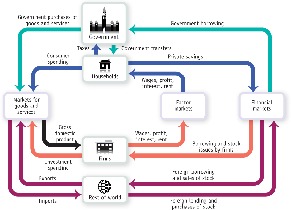
Figure 2-7 showed a simplified world containing only two kinds of “inhabitants,” households and firms. And it illustrated the circular flow of money between households and firms, which remains visible in Figure 7-1. In the markets for goods and services, households engage in consumer spending (or consumption), buying goods and services from domestic firms and from firms in the rest of the world. Households also own factors of production—labour, land, physical capital, human capital, and financial capital. They sell the use of these factors of production to firms, receiving wages, profit, interest payments, and rent in return. Firms buy and pay households for the use of those factors of production in the factor markets. Most households derive the bulk of their income from wages earned by selling labour and human capital. But households derive additional income from their indirect ownership of the physical capital used by firms, mainly in the form of stocks, shares in the ownership of a company, and from bonds, by borrowing in the form of an IOU that pays interest. So the income households receive from the factor markets includes profits distributed to shareholders known as dividends, and the interest payments on bonds held by bondholders. Finally, households receive rent in return for allowing firms to use land or structures that they own. So households receive income in the form of wages, profit, interest payments, and rent via factor markets.

In our original, simplified circular-flow diagram, households spent all the income they received via factor markets on goods and services. Figure 7-1, however, illustrates a more complicated but more realistic diagram. There we see two reasons why goods and services don’t in fact absorb all of households’ income. First, households don’t get to keep all the income they receive via the factor markets. They must pay part of their income to the government in the form of taxes, such as income taxes and sales taxes. In addition, some households receive government transfers—payments by the government to individuals for which no good or service is provided in return, such as Canadian public pension benefits and employment insurance payments. The total income households have left after paying taxes and receiving government transfers is disposable income.

Second, households normally don’t spend all their disposable income on goods and services. Instead, a portion of their income is typically set aside as private savings, which goes into financial markets where individuals, banks, and other institutions buy and sell stocks and bonds as well as make loans. As Figure 7-1 shows, the financial markets also receive funds from the rest of the world and provide funds to the government, to firms, and to the rest of the world.

Before going further, we can use the box representing households to illustrate an important general feature of the circular-flow diagram: the total sum of flows of money out of a given box is equal to the total sum of flows of money into that box. It’s simply a matter of accounting: what goes in must come out. So, for example, the total flow of money out of households—the sum of taxes paid, consumer spending, and private savings—must equal the total flow of money into households—the sum of wages, profit, interest payments, rent, and government transfers.

Now let’s look at the other types of inhabitants we’ve added to the circular-flow diagram, including the government—all federal, provincial, and municipal governments—and the rest of the world. The government returns a portion of the money it collects from taxes to households in the form of government transfers. However, it uses much of its tax revenue, plus additional funds borrowed in the financial markets through government borrowing, to buy goods and services. Government purchases of goods and services, the total purchases by federal, provincial, and municipal governments, include everything from military spending on UN peacekeeping duties to your local public school’s spending on chalk, erasers, and teacher salaries.

The rest of the world participates in the Canadian economy in three ways:

Finally, let’s go back to the markets for goods and services. In Chapter 2 we focused only on purchases of goods and services by households. We now see that there are other types of spending on goods and services, including government purchases, investment spending by firms, imports, and exports.

Notice that firms also buy goods and services in our expanded economy. For example, an automobile company that is building a new factory will buy investment goods—machinery like stamping presses and welding robots that are used to produce goods and services for consumers—from companies that manufacture these items. It will also accumulate an inventory of finished cars in preparation for shipment to dealers. Inventories, then, are stocks of goods and raw materials that firms hold to facilitate their operations. The national accounts count this investment spending (or investment)—spending on productive physical capital, such as on new machinery and equipment and on construction of buildings, and on changes to inventories—as part of total spending on goods and services.

You might ask why changes to inventories are included in investment spending—finished cars aren’t, after all, used to produce more cars. Changes to inventories of finished goods are counted as investment spending because, like machinery, they change the ability of a firm to make future sales. So spending on additions to inventories is a form of investment spending by a firm. Conversely, a drawing-down of inventories is counted as a fall in investment spending because it leads to lower future sales. It’s also important to understand that investment spending includes spending on construction of any structure, regardless of whether it is an assembly plant or a new house. Why include construction of homes? Because, like a plant, a new house produces a future stream of output—housing services for its occupants.

Suppose we add up consumer spending on goods and services, investment spending, government purchases of goods and services, and the value of exports, and then subtract the value of imports. This gives us a measure of the overall market value of the goods and services the economy produces. That measure has a name: it’s a country’s gross domestic product. But before we can formally define gross domestic product, or GDP, we have to examine an important distinction between classes of goods and services: the difference between final goods and services versus intermediate goods and services.

A consumer’s purchase of a new car from a dealer is one example of a sale of final goods and services: goods and services sold to the final, or end, user. But an automobile manufacturer’s purchase of steel from a steel foundry or glass from a glassmaker is an example of purchasing intermediate goods and services: goods and services that are inputs for production of other goods and services. In the case of intermediate goods and services, the purchaser—another firm—is not the final user.

Gross domestic product, or GDP, is the total value of all final goods and services produced in an economy during a given period, usually a year. In 2011, the GDP in Canada was $1721 billion, or about $49 902 per person. If you are an economist trying to construct a country’s national accounts, one way to calculate GDP is to calculate it directly: survey firms and add up the total value of their production of final goods and services. We’ll explain in detail in the next section why intermediate goods, and some other types of goods as well, are not included in the calculation of GDP.

But adding up the total value of final goods and services produced isn’t the only way of calculating GDP. There is another way, based on total spending on final goods and services. Since GDP is equal to the total value of final goods and services produced in the economy, it must also equal the flow of funds received by firms from sales in the goods and services market.

If you look again at the circular-flow diagram in Figure 7-1, you will see that the arrow going from markets for goods and services to firms is indeed labelled “Gross domestic product.” According to our basic rule of accounting, flows out of any box are equal to flows into the box; so the flow of funds out of the markets for goods and services to firms is equal to the total flow of funds into the markets for goods and services from other sectors. And as you can see from Figure 7-1, the total flow of funds into the markets for goods and services is total or aggregate expenditure on domestically produced final goods and services—the sum of consumer spending, investment spending, government purchases of goods and services, and exports minus imports. So a second way of calculating GDP is to add up aggregate expenditure on domestically produced final goods and services in the economy.

And there is yet a third way of calculating GDP, based on total income earned by factors of production (inputs) in the economy. Firms, and the factors of production that they employ, are owned by households. So firms must ultimately pay out what they earn to households. The flow from firms to the factor markets is the factor income paid out by firms to households in the form of wages, profit, interest, and rent. Again, by accounting rules, the value of the flow of factor income from firms to households must be equal to the flow of money into firms from the markets for goods and services. And this last value, we know, is the total value of production in the economy—GDP. Why is GDP equal to the total value of factor income paid by firms in the economy to households? Because each sale in the economy must accrue to someone as income—either as wages, profit, interest, or rent. So a third way of calculating GDP is to add up all the factor income earned by households from firms in the economy.

We’ve just explained that there are in fact three methods for calculating GDP:

Government statisticians use all three methods. To illustrate how these three methods work, we will consider a hypothetical economy, shown in Figure 7-2. This economy consists of three firms—Canadian Motors, Inc., which produces one car per year; Canadian Steel, Inc., which produces the steel that goes into the car; and Canadian Ore, Inc., which mines the iron ore that goes into the steel. So GDP is $21 500, the value of the one car per year the economy produces. Let’s look at how the three different methods of calculating GDP yield the same result.

The Value-Added Approach: Measuring GDP as the Value of Production of Final Goods and Services The first method for calculating GDP is to add up the value of all the final goods and services produced in the economy—a calculation that excludes the value of intermediate goods and services. Why are intermediate goods and services excluded? After all, don’t they represent a very large and valuable portion of the economy?

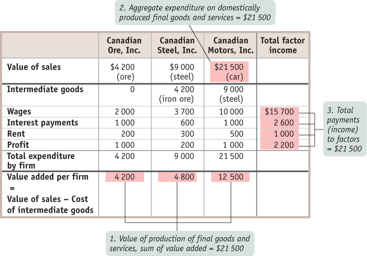
To understand why only final goods and services are included in GDP, look at the simplified economy described in Figure 7-2. Should we measure the GDP of this economy by adding up the total sales of the iron ore producer, the steel producer, and the auto producer? If we did, we would in effect be counting the value of the steel twice—once when it is sold by the steel plant to the auto plant, and again when the steel auto body is sold to a consumer as a finished car. And we would be counting the value of the iron ore three times—once when it is mined and sold to the steel company, a second time when it is made into steel and sold to the auto producer, and a third time when the steel is made into a car and sold to the consumer.

So counting the full value of each producer’s sales would cause us to count the same items several times and artificially inflate the calculation of GDP. For example, in Figure 7-2, the total value of all sales, intermediate and final, is $34700: $21500 from the sale of the car, plus $9000 from the sale of the steel, plus $4200 from the sale of the iron ore. Yet we know that GDP is only $21500. The way we avoid double-counting is to count only each producer’s value added in the calculation of GDP: the difference between the value of its sales and the value of the intermediate goods and services it purchases from other businesses.

That is, at each stage of the production process we subtract the cost of inputs—the intermediate goods—at that stage. In this case, the value added of the auto producer is the dollar value of the cars it manufactures minus the cost of the steel it buys, or $12500. The value added of the steel producer is the dollar value of the steel it produces minus the cost of the ore it buys, or $4800. Only the ore producer, which we have assumed doesn’t buy any inputs, has value added equal to its total sales, $4200. The sum of the three producers’ value added is $21500, equal to GDP.

In Canada, the value added of goods-producing industries such as manufacturing, construction, and resource extraction account for about 30% of GDP; while the valued added of service-producing industries such as financial and health care industries account for the remaining 70%.

The “Our Imputed Lives” box below discusses the important assumptions the government makes to estimate the value added of households.

The Expenditure Approach: Measuring GDP as Spending on Domestically Produced Final Goods and Services Another way to calculate GDP is by adding up aggregate expenditure on domestically produced final goods and services. That is, GDP can be measured by the flow of funds into firms. Like the method that estimates GDP as the value of domestic production of final goods and services, this measurement must be carried out in a way that avoids double-counting. In terms of our steel and auto example, we don’t want to count both consumer spending on a car (represented in Figure 7-2 by $21500, the sales price of the car) and the auto producer’s spending on steel (represented in Figure 7-2 by $9000, the price of a car’s worth of steel). If we counted both, we would be counting the steel embodied in the car twice. We solve this problem by counting only the value of sales to final buyers, such as consumers, firms that purchase investment goods, the government, or foreign buyers. In other words, in order to avoid double-counting of spending, we omit sales of inputs from one business to another when estimating GDP using spending data. You can see from Figure7-2 that aggregate expenditure on final goods and services—the finished car—is $21500.

As we’ve already pointed out, the national accounts do include investment spending by firms as a part of final spending. That is, an auto company’s purchase of steel to make a car isn’t considered a part of final spending, but the company’s purchase of new machinery for its factory is considered a part of final spending. What’s the difference? Steel is an input that is used up in production; machinery will last for a number of years. Since purchases of capital goods that will last for a considerable time aren’t closely tied to current production, the national accounts consider such purchases a form of final sales.

In later chapters, we will make use of the proposition that GDP is equal to aggregate expenditure on domestically produced goods and services by final buyers. We will also develop models of how final buyers decide how much to spend. With that in mind, we’ll now examine the types of spending that make up GDP.

Look again at the markets for goods and services in Figure 7-1, and you will see that one component of sales by firms is consumer spending. Let’s denote consumer spending with the symbol C. Figure 7-1 also shows three other components of sales: sales of investment goods to other businesses, or investment spending, which we will denote by I; government purchases of goods and services, which we will denote by G; and sales to foreigners—that is, exports—which we will denote by X.

In reality, not all of this final spending goes toward domestically produced goods and services. We must take account of spending on imports, which we will denote by IM. Income spent on imports is income not spent on domestic goods and services—it is income that has “leaked” across national borders. So to accurately value domestic production using spending data, we must subtract spending on imports to arrive at spending on domestically produced goods and services. Putting this all together gives us the following equation that breaks GDP down by the four sources of aggregate expenditure:

We’ll be seeing a lot of Equation 7-1 in later chapters.

The Income Approach: Measuring GDP as Income Earned from Production of Goods and Services A final way to calculate GDP is to add two sources of income: factor incomes and non-factor payments. Factor incomes consist of the income earned by factors of production, or inputs. Examples include the wages earned by workers; the interest paid to those who lend their savings to firms; the rent earned by those who lease their land or structures to firms; the dividends paid to shareholders, who own a firm’s physical capital; and other income earned by those who are directly involved in the production of goods and services.

Non-factor payments consist of the income earned by the federal government as a result of the production of goods and services. They are the difference between the prices for which final products are sold in the market and the amount actually received (and kept) by the factors of production before income taxes are removed. One example is net indirect taxes, which are indirect taxes, such as provincial and federal sales taxes, less any subsidies paid to purchasers. Another example is capital depreciation, which is the removal of productive physical capital from the capital stock as it wears out or becomes obsolete; such depreciation can be claimed as an income tax deduction.

Figure 7-2 shows how this calculation works for our simplified economy. The shaded column at the far right shows the total wages, interest, and rent paid by all these firms as well as their total profit. Summing up all of these yields total factor income of $21500—again, equal to GDP.

Here, we’ll focus on the expenditure approach and the income approach in calculating GDP. It’s important to keep in mind, however, that all the money spent on domestically produced goods and services generates income for someone in the economy because one person’s spending is another person’s income—that is, there really is a circular flow. Figure 7-3 shows that the economy’s total expenditure must equal its total income.

The Components of GDP Now that we know how GDP is calculated in principle, let’s see what it looks like in practice.

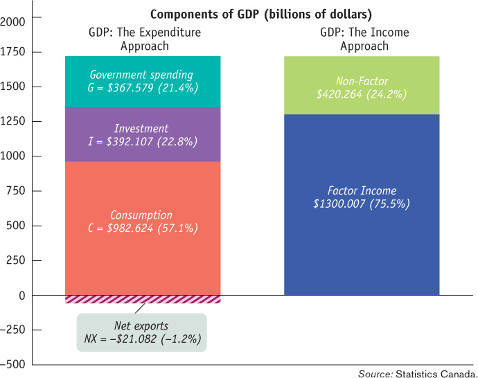
Figure 7-3 shows the last two methods of calculating GDP side by side. The height of each bar above the horizontal axis represents the GDP of the Canadian economy in 2011: $1721 billion. Each bar is divided to show the breakdown of that total in terms of where the value was added, how the money was spent, and where the income was generated.

The left bar in Figure 7-3 corresponds to the second method of calculating GDP, showing the breakdown by the four types of aggregate expenditure. The total length of the bar on the left is longer than the bar on the right, a difference of $21 billion (which, as you can see, is the amount by which the left bar extends below the horizontal axis). That’s because the total length of the left bar represents total spending in the economy, spending on both domestically produced and foreign-produced final goods and services. Within the bar, consumer spending (C), which is 57.1% of GDP, dominates the picture. But some of that spending was absorbed by foreign-produced goods and services. In 2011, net exports, the difference between the value of exports and the value of imports (X − IM in Equation 7-1) was negative—Canada was a net importer of foreign goods and services. The 2011 value of X − IM was −$21.1 billion, or −1.2% of GDP. Thus, a portion of the left bar extends below the horizontal axis by $21.1 billion to represent the amount of total spending that was absorbed by net imports and so did not lead to higher Canadian GDP. Investment spending (I) constituted 22.8% of GDP; government purchases of goods and services (G) constituted 21.4% of GDP.

The bar on the right shows Canada’s GDP calculated according to the income approach. About 76% of Canada’s GDP in 2011, or about $1300 billion, consisted of factor incomes. Of that amount, the labour force earned $889.5 billion, the firms’ owners made $366.7 billion, and the owners of capital made $73.8 billion. The remainder of the 2011 GDP, about 24%, or $420.3 billion, comprised non-factor payments, such as the net indirect taxes collected by governments plus the amount of capital depreciation. Adding both numbers yields the incomes estimate of GDP, which in 2011 was 1720.3 billion. This is slightly less than the reported GDP of $1720.748 billion. The difference is due to statistical discrepancy.

Now we’ve seen the various ways that gross domestic product is calculated. But what does the measurement of GDP tell us?

The most important use of GDP is as a measure of the size of the economy, providing us a scale against which to measure the economic performance of other years or to compare the economic performance of other countries. For example, suppose you want to compare the economies of different nations. A natural approach is to compare their GDPs. In 2011, as we’ve seen, Canada’s GDP was quite large: $1721 billion. But China’s GDP was $7126 billion, the U.S. had the biggest national economy at $14 928 billion, and the European Union’s GDP was $16 488 billion. (All figures in Canadian dollars.) This comparison tells us that China, although it has the world’s second-largest national economy, carries considerably less economic weight than does the United States. Canada’s economy is about one-tenth of the size of the American economy. When taken in aggregate, the European Union, which consists of 28 countries, is America’s equal or superior.

Still, one must be careful when using GDP numbers, especially when making comparisons over time. That’s because part of the increase in the value of GDP over time represents increases in the prices of goods and services rather than an increase in output. For example, from 1992 to 2011, Canada’s GDP increased in size about 2.5 times, from $700 billion to $1721 billion. But the Canadian economy did not really increase by 2.5 times over that period. To measure actual changes in aggregate output, we need a modified version of GDP that is adjusted for price changes, known as real GDP. We’ll see next how real GDP is calculated.

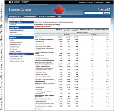
The CSNA includes numerous related items, such as the Monthly Retail Trade Survey (MRTS). Retail sales are an important component of gross domestic product, which is a key indicator of consumer purchasing patterns in Canada. This information is valuable to many organizations. Federal and provincial governments use it to gain an understanding of the overall economy and to design tax and spending policies. The Bank of Canada uses it to decide on monetary policy. For example, high retail sales could suggest to the federal government that its economic stimulus programs have been successful and could suggest to the Bank of Canada that it should consider raising interest rates. A business can use this information to compare its own sales performance against the industry standard. Investors may use it to decide whether to invest in a certain industry or not.