Inflation and Unemployment in the Long Run
The short-
However, this view was greatly altered by the later recognition that expected inflation affects the short-
So what does the trade-
The Long-Run Phillips Curve
Figure 31-12 reproduces the two short-
31-12
The NAIRU and the Long-
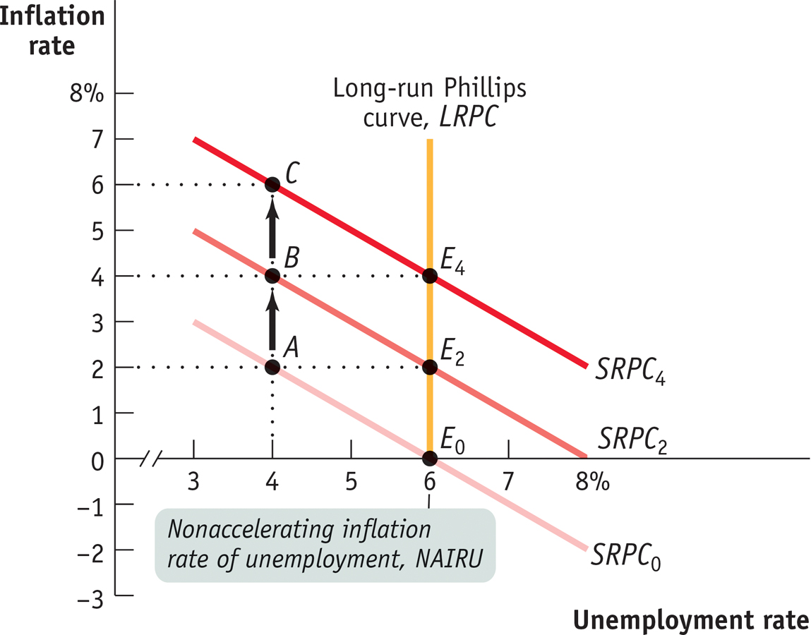
Suppose that the economy has, in the past, had a 0% inflation rate. In that case, the current short-
Also suppose that policy makers decide to trade off lower unemployment for a higher rate of inflation. They use monetary policy, fiscal policy, or both to drive the unemployment rate down to 4%. This puts the economy at point A on SRPC0, leading to an actual inflation rate of 2%.
Over time, the public will come to expect a 2% inflation rate. This increase in inflationary expectations will shift the short-
Eventually, the 4% actual inflation rate gets built into expectations about the future inflation rate, and the short-
To avoid accelerating inflation over time, the unemployment rate must be high enough that the actual rate of inflation matches the expected rate of inflation. This is the situation at E0 on SRPC0: when the expected inflation rate is 0% and the unemployment rate is 6%, the actual inflation rate is 0%. It is also the situation at E2 on SRPC2: when the expected inflation rate is 2% and the unemployment rate is 6%, the actual inflation rate is 2%. And it is the situation at E4 on SRPC4: when the expected inflation rate is 4% and the unemployment rate is 6%, the actual inflation rate is 4%. As we’ll learn in Chapter 33, this relationship between accelerating inflation and the unemployment rate is known as the natural rate hypothesis.
The nonaccelerating inflation rate of unemployment, or NAIRU, is the unemployment rate at which inflation does not change over time.
The unemployment rate at which inflation does not change over time—
The long-
We can now explain the significance of the vertical line LRPC. It is the long-
The Natural Rate of Unemployment, Revisited
Recall the concept of the natural rate of unemployment, the portion of the unemployment rate unaffected by the swings of the business cycle. Now we have introduced the concept of the NAIRU. How do these two concepts relate to each other?
The answer is that the NAIRU is another name for the natural rate. The level of unemployment the economy “needs” in order to avoid accelerating inflation is equal to the natural rate of unemployment.
In fact, economists estimate the natural rate of unemployment by looking for evidence about the NAIRU from the behavior of the inflation rate and the unemployment rate over the course of the business cycle. For example, the way major European countries learned, to their dismay, that their natural rates of unemployment were 9% or more was through unpleasant experience. In the late 1980s, and again in the late 1990s, European inflation began to accelerate as European unemployment rates, which had been above 9%, began to fall, approaching 8%.
In Figure 31-4 we cited Congressional Budget Office estimates of the U.S. natural rate of unemployment. The CBO has a model that predicts changes in the inflation rate based on the deviation of the actual unemployment rate from the natural rate. Given data on actual unemployment and inflation, this model can be used to deduce estimates of the natural rate—
The Costs of Disinflation
Through experience, policy makers have found that bringing inflation down is a much harder task than increasing it. The reason is that once the public has come to expect continuing inflation, bringing inflation down is painful.
| Disinflation Around the World |
The great disinflation of the 1980s wasn’t unique to the United States. A number of other advanced countries also experienced high inflation during the 1970s, then brought inflation down during the 1980s at the cost of a severe recession. This figure shows the annual rate of inflation in Britain, Italy, and the United States from 1970 to 2013. All three nations experienced high inflation rates following the two oil price shocks of 1973 and 1979, with the U.S. inflation rate the least severe of the three. All three nations then weathered severe recessions in order to bring inflation down. Since the 1980s, inflation has remained low and stable in all wealthy nations.
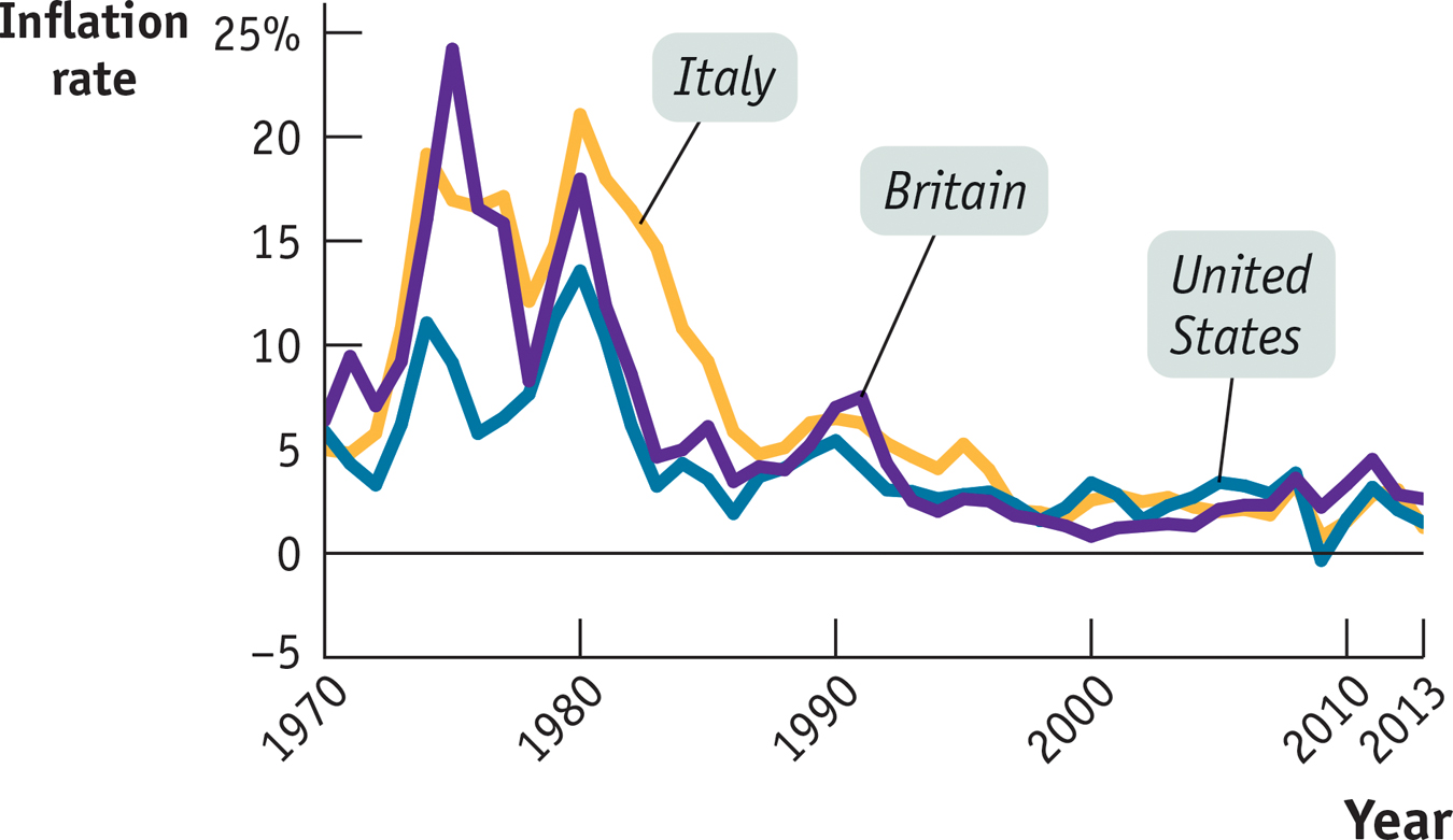
Source: OECD.
A persistent attempt to keep unemployment below the natural rate leads to accelerating inflation that becomes incorporated into expectations. To reduce inflationary expectations, policy makers need to run the process in reverse, adopting contractionary policies that keep the unemployment rate above the natural rate for an extended period of time. The process of bringing down inflation that has become embedded in expectations is known as disinflation, a concept we learned about in Chapter 23.
Disinflation can be very expensive. As the following Economics in Action documents, the U.S. retreat from high inflation at the beginning of the 1980s appears to have cost the equivalent of about 18% of a year’s real GDP, the equivalent of roughly $2.6 trillion today. The justification for paying these costs is that they lead to a permanent gain. Although the economy does not recover the short-
Some economists argue that the costs of disinflation can be reduced if policy makers explicitly state their determination to reduce inflation. A clearly announced, credible policy of disinflation, they contend, can reduce expectations of future inflation and so shift the short-
ECONOMICS in Action: The Great Disinflation of the 1980s
The Great Disinflation of the 1980s
As we’ve mentioned several times in this chapter, the United States ended the 1970s with a high rate of inflation, at least by its own peacetime historical standards—
31-13
The Great Disinflation
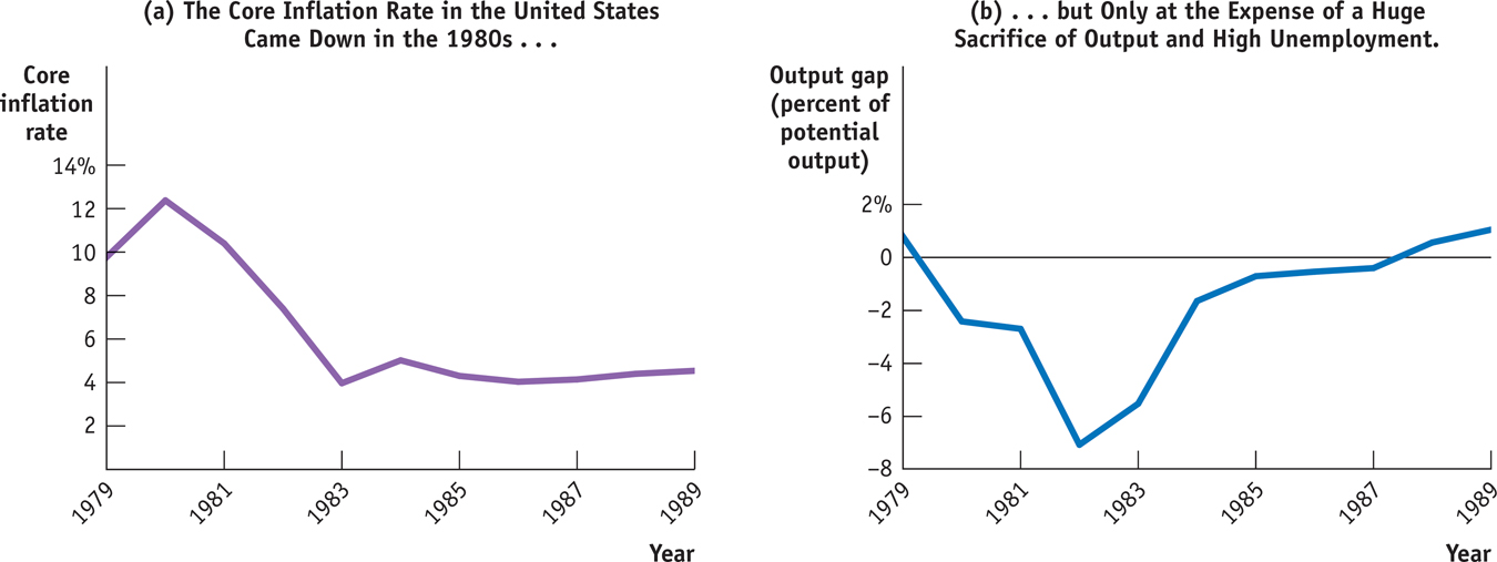
By the mid-
How was this disinflation achieved? At great cost. Beginning in late 1979, the Federal Reserve imposed strongly contractionary monetary policies, which pushed the economy into its worst recession since the Great Depression. Panel (b) shows the Congressional Budget Office estimate of the U.S. output gap from 1979 to 1989: by 1982, actual output was 7% below potential output, corresponding to an unemployment rate of more than 9%. Aggregate output didn’t get back to potential output until 1987.
Our analysis of the Phillips curve tells us that a temporary rise in unemployment, like that of the 1980s, is needed to break the cycle of inflationary expectations. Once expectations of inflation are reduced, the economy can return to the natural rate of unemployment at a lower inflation rate. And that’s just what happened.
But the cost was huge. If you add up the output gap over 1980–
Quick Review
Policies that keep the unemployment rate below the NAIRU, the nonaccelerating rate of inflation, will lead to accelerating inflation as inflationary expectations adjust to higher levels of actual inflation. The NAIRU is equal to the natural rate of unemployment.
The long-
run Phillips curve is vertical and shows that an unemployment rate below the NAIRU cannot be maintained in the long run. As a result, there are limits to expansionary policies.Disinflation imposes high costs—
unemployment and lost output— on an economy. Governments do it to avoid the costs of persistently high inflation.
31-3
Question 16.5
Why is there no long-
run trade- off between unemployment and inflation? There is no long-run trade-off between inflation and unemployment because once expectations of inflation adjust, wages will also adjust, returning employment and the unemployment rate to their equilibrium (natural) levels. This implies that once expectations of inflation fully adjust to any change in actual inflation, the unemployment rate will return to the natural rate of unemployment, or NAIRU. This also implies that the long-run Phillips curve is vertical.
Question 16.6
British economists believe that the natural rate of unemployment in that country rose sharply during the 1970s, from around 3% to as much as 10%. During that period, Britain experienced a sharp acceleration of inflation, which for a time went above 20%. How might these facts be related?
There are two possible explanations for this. First, negative supply shocks (for example, increases in the price of oil) will cause an increase in unemployment and an increase in inflation. Second, it is possible that British policy makers attempted to peg the unemployment rate below the natural rate of unemployment. Any attempt to peg unemployment below the natural rate will result in an increase in inflation.
Question 16.7
Why is disinflation so costly for an economy? Are there ways to reduce these costs?
Disinflation is costly because to reduce the inflation rate, aggregate output in the short run must typically fall below potential output. This, in turn, results in an increase in the unemployment rate above the natural rate. In general, we would observe a reduction in real GDP. The costs of disinflation can be reduced by not allowing inflation to increase in the first place. Second, the costs of any disinflation will be lower if the central bank is credible and it announces in advance its policy to reduce inflation. In this situation, the adjustment to the disinflationary policy will be more rapid, resulting in a smaller loss of aggregate output.
Solutions appear at back of book.