16.2 Aggregate Demand
The aggregate demand curve shows the relationship between the aggregate price level and the quantity of aggregate output demanded by households, businesses, the government, and the rest of the world.
The Great Depression, the great majority of economists agree, was the result of a massive negative demand shock. What does that mean? In Chapter 3 we explained that when economists talk about a fall in the demand for a particular good or service, they’re referring to a leftward shift of the demand curve. Similarly, when economists talk about a negative demand shock to the economy as a whole, they’re referring to a leftward shift of the aggregate demand curve, a curve that shows the relationship between the aggregate price level and the quantity of aggregate output demanded by households, firms, the government, and the rest of the world.
Figure 16-1 shows what the aggregate demand curve may have looked like in 1933, at the end of the 1929–1933 recession. The horizontal axis shows the total quantity of domestic goods and services demanded, measured in 2009 dollars. We use real GDP to measure aggregate output and will often use the two terms interchangeably. The vertical axis shows the aggregate price level, measured by the GDP deflator. With these variables on the axes, we can draw a curve, AD, showing how much aggregate output would have been demanded at any given aggregate price level. Since AD is meant to illustrate aggregate demand in 1933, one point on the curve corresponds to actual data for 1933, when the aggregate price level was 7.3 and the total quantity of domestic final goods and services purchased was $778 billion in 2009 dollars.
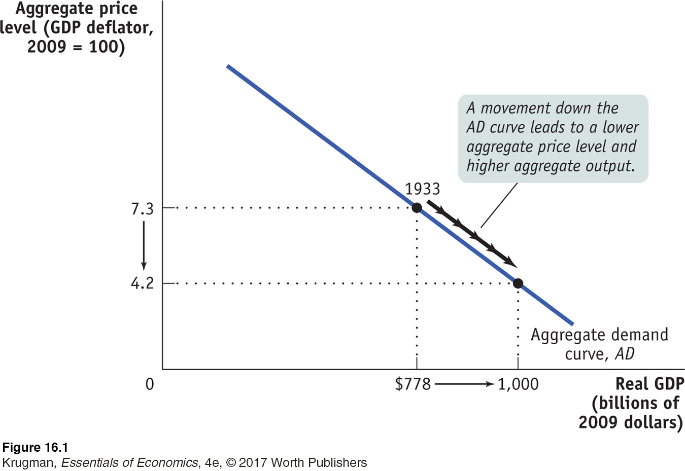
As drawn in Figure 16-1, the aggregate demand curve is downward sloping, indicating a negative relationship between the aggregate price level and the quantity of aggregate output demanded. A higher aggregate price level, other things equal, reduces the quantity of aggregate output demanded; a lower aggregate price level, other things equal, increases the quantity of aggregate output demanded. According to Figure 16-1, if the price level in 1933 had been 4.2 instead of 7.3, the total quantity of domestic final goods and services demanded would have been $1,000 billion in 2009 dollars instead of $778 billion.
The first key question about the aggregate demand curve is: why should the curve be downward sloping?
Why Is the Aggregate Demand Curve Downward Sloping?
In Figure 16-1, the curve AD is downward sloping. To understand why, you’ll need to learn the basic equation of national income accounting:
(16-
where C is consumer spending, I is investment spending, G is government purchases of goods and services, X is exports to other countries, and IM is imports. If we measure these variables in constant dollars—
You might think that the downward slope of the aggregate demand curve is a natural consequence of the law of demand we defined back in Chapter 3. That is, since the demand curve for any one good is downward sloping, isn’t it natural that the demand curve for aggregate output is also downward sloping? This turns out, however, to be a misleading parallel. The demand curve for any individual good shows how the quantity demanded depends on the price of that good, holding the prices of other goods and services constant. The main reason the quantity of a good demanded falls when the price of that good rises—
But when we consider movements up or down the aggregate demand curve, we’re considering a simultaneous change in the prices of all final goods and services. Furthermore, changes in the composition of goods and services in consumer spending aren’t relevant to the aggregate demand curve: if consumers decide to buy fewer clothes but more cars, this doesn’t necessarily change the total quantity of final goods and services they demand.
Why, then, does a rise in the aggregate price level lead to a fall in the quantity of all domestically produced final goods and services demanded? There are two main reasons: the wealth effect and the interest rate effect of a change in the aggregate price level.
The Wealth Effect An increase in the aggregate price level, other things equal, reduces the purchasing power of many assets. Consider, for example, someone who has $5,000 in a bank account. If the aggregate price level were to rise by 25%, what used to cost $5,000 would now cost $6,250, and would no longer be affordable. And what used to cost $4,000 would now cost $5,000, so that the $5,000 in the bank account would now buy only as much as $4,000 would have bought previously. With the loss in purchasing power, the owner of that bank account would probably scale back his or her consumption plans. Millions of other people would respond the same way, leading to a fall in spending on final goods and services, because a rise in the aggregate price level reduces the purchasing power of everyone’s bank account.
The wealth effect of a change in the aggregate price level is the effect on consumer spending caused by the effect of a change in the aggregate price level on the purchasing power of consumers’ assets.
Correspondingly, a fall in the aggregate price level increases the purchasing power of consumers’ assets and leads to more consumer demand. The wealth effect of a change in the aggregate price level is the effect on consumer spending caused by the effect of a change in the aggregate price level on the purchasing power of consumers’ assets. Because of the wealth effect, consumer spending, C, falls when the aggregate price level rises, leading to a downward-
PITFALLS
CHANGES IN WEALTH: A MOVEMENT ALONG VERSUS A SHIFT OF THE AGGREGATE DEMAND CURVE
Earlier we explained that one reason the AD curve is downward sloping is the wealth effect of a change in the aggregate price level: a higher aggregate price level reduces the purchasing power of households’ assets and leads to a fall in consumer spending, C. But we’ve just explained that changes in wealth lead to a shift of the AD curve. Aren’t those two explanations contradictory? Which one is it—
A movement along the AD curve occurs when a change in the aggregate price level changes the purchasing power of consumers’ existing wealth (the real value of their assets). This is the wealth effect of a change in the aggregate price level—
In contrast, a change in wealth independent of a change in the aggregate price level shifts the AD curve. So, a rise in the stock market or in real estate values leads to an increase in the real value of consumers’ assets at any given aggregate price level. In this case, the source of the change in wealth is a change in the values of assets without any change in the aggregate price level—
The Interest Rate Effect Economists use the term money in its narrowest sense to refer to cash and bank deposits on which people can write checks. People and firms hold money because it reduces the cost and inconvenience of making transactions. An increase in the aggregate price level, other things equal, reduces the purchasing power of a given amount of money holdings. To purchase the same basket of goods and services as before, people and firms now need to hold more money. So, in response to an increase in the aggregate price level, the public tries to increase its money holdings, either by borrowing more or by selling assets such as bonds. This reduces the funds available for lending to other borrowers and drives interest rates up.
The interest rate effect of a change in the aggregate price level is the effect on consumer spending and investment spending caused by the effect of a change in the aggregate price level on the purchasing power of consumers’ and firms’ money holdings.
A rise in the interest rate reduces investment spending because it makes the cost of borrowing higher. It also reduces consumer spending because households save more of their disposable income. So a rise in the aggregate price level depresses investment spending, I, and consumer spending, C, through its effect on the purchasing power of money holdings, an effect known as the interest rate effect of a change in the aggregate price level. This also leads to a downward-
We’ll have a lot more to say about money and interest rates in Chapter 19 on monetary policy. For now, the important point is that the aggregate demand curve is downward sloping due to both the wealth effect and the interest rate effect of a change in the aggregate price level.
Shifts of the Aggregate Demand Curve
In Chapter 3, where we introduced the analysis of supply and demand in the market for an individual good, we stressed the importance of the distinction between movements along the demand curve and shifts of the demand curve. The same distinction applies to the aggregate demand curve. Figure 16-1 shows a movement along the aggregate demand curve, a change in the aggregate quantity of goods and services demanded as the aggregate price level changes.
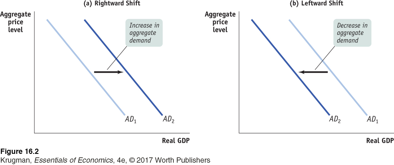
But there can also be shifts of the aggregate demand curve, changes in the quantity of goods and services demanded at any given price level, as shown in Figure 16-2. When we talk about an increase in aggregate demand, we mean a shift of the aggregate demand curve to the right, as shown in panel (a) by the shift from AD1 to AD2. A rightward shift occurs when the quantity of aggregate output demanded increases at any given aggregate price level. A decrease in aggregate demand means that the AD curve shifts to the left, as in panel (b). A leftward shift implies that the quantity of aggregate output demanded falls at any given aggregate price level.
A number of factors can shift the aggregate demand curve. Among the most important are changes in expectations, changes in wealth, and the size of the existing stock of physical capital. In addition, both fiscal and monetary policy can shift the aggregate demand curve. We’ll now examine each of the factors that shift the aggregate demand curve. For an overview of them, see Table 16-1.
| When this happens, . . . |
. . . aggregate demand increases: |
But when this happens, . . . |
. . . aggregate demand decreases: |
| Changes in expectations: | |||

|
|
||
| Changes in wealth: | |||
|
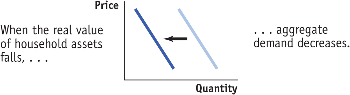
|
||
| Size of the existing stock of physical capital: | |||
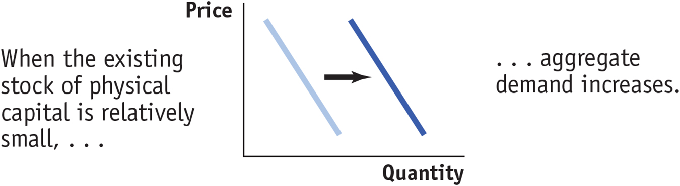
|

|
||
| Fiscal policy: | |||
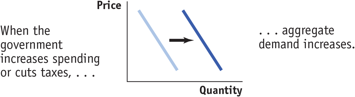
|
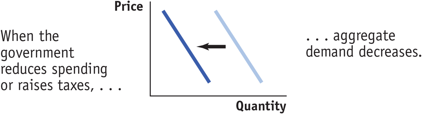
|
||
| Monetary policy: | |||
|
|
||
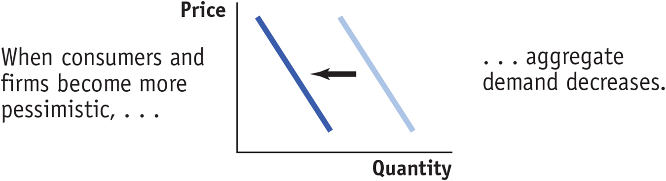
Changes in Expectations Both consumer spending and planned investment spending depend in part on people’s expectations about the future. Consumers base their spending not only on the income they have now but also on the income they expect to have in the future. Firms base their planned investment spending not only on current conditions but also on the sales they expect to make in the future. As a result, changes in expectations can push consumer spending and planned investment spending up or down. If consumers and firms become more optimistic, aggregate spending rises; if they become more pessimistic, aggregate spending falls.
In fact, short-
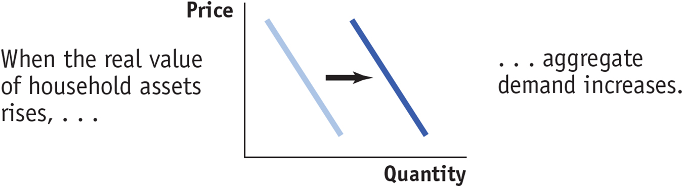
Changes in Wealth Consumer spending depends in part on the value of household assets. When the real value of these assets rises, the purchasing power they embody also rises, leading to an increase in aggregate spending. For example, in the 1990s there was a significant rise in the stock market that increased aggregate demand. And when the real value of household assets falls—
Size of the Existing Stock of Physical Capital Firms engage in planned investment spending to add to their stock of physical capital. Their incentive to spend depends in part on how much physical capital they already have: the more they have, the less they will feel a need to add more, other things equal. The same applies to other types of investment spending—
Government Policies and Aggregate Demand
One of the key insights of macroeconomics is that the government can have a powerful influence on aggregate demand and that, in some circumstances, this influence can be used to improve economic performance.
The two main ways the government can influence the aggregate demand curve are through fiscal policy and monetary policy. We’ll briefly discuss their influence on aggregate demand, leaving a full-
Fiscal Policy As we learned, fiscal policy is the use of either government spending—
The effect of government purchases of final goods and services, G, on the aggregate demand curve is direct because government purchases are themselves a component of aggregate demand. So an increase in government purchases shifts the aggregate demand curve to the right and a decrease shifts it to the left. History’s most dramatic example of how increased government purchases affect aggregate demand was the effect of wartime government spending during World War II.
Because of the war, U.S. federal purchases surged 400%. This increase in purchases is usually credited with ending the Great Depression. In the 1990s Japan used large public works projects—
In contrast, changes in either tax rates or government transfers influence the economy indirectly through their effect on disposable income. A lower tax rate means that consumers get to keep more of what they earn, increasing their disposable income. An increase in government transfers also increases consumers’ disposable income. In either case, this increases consumer spending and shifts the aggregate demand curve to the right. A higher tax rate or a reduction in transfers reduces the amount of disposable income received by consumers. This reduces consumer spending and shifts the aggregate demand curve to the left.
Monetary Policy Earlier we talked about the problems faced by the FOMC, the branch of the Federal Reserve that controls monetary policy—
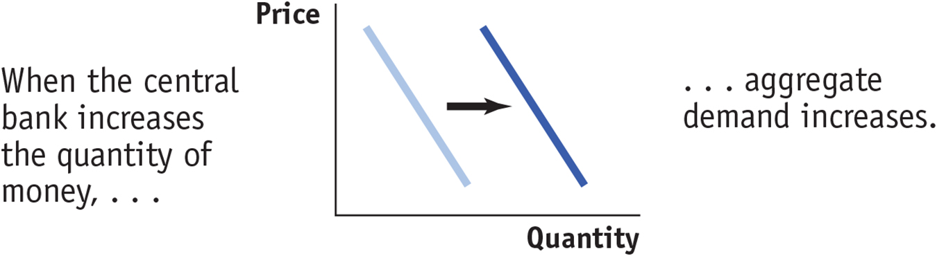
But what happens if the quantity of money in the hands of households and firms changes? In modern economies, the quantity of money in circulation is largely determined by the decisions of a central bank created by the government. As we’ll learn in Chapter 18, the Federal Reserve, the U.S. central bank, is a special institution that is neither exactly part of the government nor exactly a private institution. When the central bank increases the quantity of money in circulation, households and firms have more money, which they are willing to lend out. The effect is to drive the interest rate down at any given aggregate price level, leading to higher investment spending and higher consumer spending.
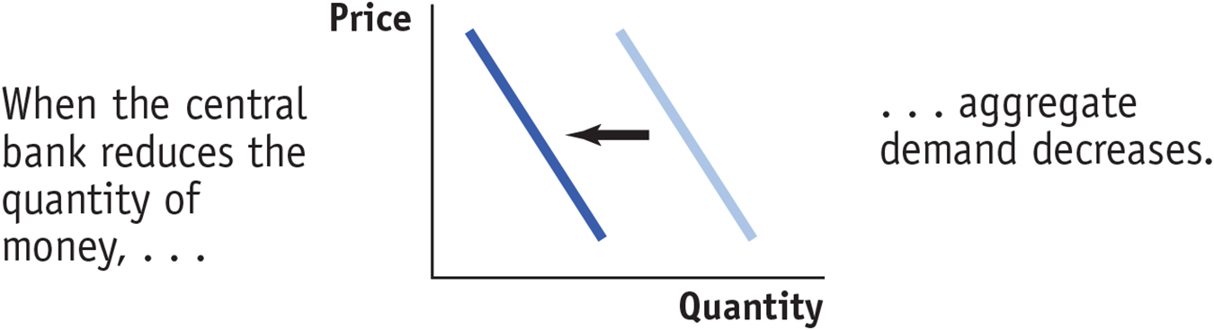
That is, increasing the quantity of money shifts the aggregate demand curve to the right. Reducing the quantity of money has the opposite effect: households and firms have less money holdings than before, leading them to borrow more and lend less. This raises the interest rate, reduces investment spending and consumer spending, and shifts the aggregate demand curve to the left.
ECONOMICSin Action
Moving Along the Aggregrate Demand Curve, 1979–1980
![]() | interactive activity
| interactive activity
When looking at data, it’s often hard to distinguish between changes in spending that represent movements along the aggregate demand curve and shifts of the aggregate demand curve. One telling exception, however, is what happened right after the oil crisis of 1979, which we mentioned in this chapter’s opening story. Faced with a sharp increase in the aggregate price level—
This led to an increase in the demand for borrowing and a surge in interest rates. The prime rate, which is the interest rate banks charge their best customers, climbed above 20%. High interest rates, in turn, caused both consumer spending and investment spending to fall: in 1980 purchases of durable consumer goods like cars fell by 5.3% and real investment spending fell by 8.9%.
In other words, in 1979–1980 the economy responded just as we’d expect if it were moving upward along the aggregate demand curve from right to left: due to the wealth effect and the interest rate effect of a change in the aggregate price level, the quantity of aggregate output demanded fell as the aggregate price level rose. This does not explain, of course, why the aggregate price level rose. But as we’ll see in the upcoming section on the AD–AS model, the answer to that question lies in the behavior of the short-
Quick Review
The aggregate demand curve is downward sloping because of the wealth effect of a change in the aggregate price level and the interest rate effect of a change in the aggregate price level.
Changes in consumer spending caused by changes in wealth and expectations about the future shift the aggregate demand curve. Changes in investment spending caused by changes in expectations and by the size of the existing stock of physical capital also shift the aggregate demand curve.
Fiscal policy affects aggregate demand directly through government purchases and indirectly through changes in taxes or government transfers. Monetary policy affects aggregate demand indirectly through changes in the interest rate.
Check Your Understanding16-1
Question 16.1
1. Determine the effect on aggregate demand of each of the following events. Explain whether it represents a movement along the aggregate demand curve (up or down) or a shift of the curve (leftward or rightward).
A rise in the interest rate caused by a change in monetary policy
This is a shift of the aggregate demand curve. A decrease in the quantity of money raises the interest rate, since people now want to borrow more and lend less. A higher interest rate reduces investment and consumer spending at any given aggregate price level. So the aggregate demand curve shifts to the left.
A fall in the real value of money in the economy due to a higher aggregate price level
This is a movement up along the aggregate demand curve. As the aggregate price level rises, the real value of money holdings falls. This is the interest rate effect of a change in the aggregate price level: as the value of money falls, people want to hold more money. They do so by borrowing more and lending less. This leads to a rise in the interest rate and a reduction in consumer and investment spending. So it is a movement along the aggregate demand curve.
News of a worse-
than- expected job market next year This is a shift of the aggregate demand curve. Expectations of a poor job market, and so lower average disposable incomes, will reduce people’s consumer spending today at any given aggregate price level. So the aggregate demand curve shifts to the left.
A fall in tax rates
This is a shift of the aggregate demand curve. A fall in tax rates raises people’s disposable income. At any given aggregate price level, consumer spending is now higher. So the aggregate demand curve shifts to the right.
A rise in the real value of assets in the economy due to a lower aggregate price level
This is a movement down along the aggregate demand curve. As the aggregate price level falls, the real value of assets rises. This is the wealth effect of a change in the aggregate price level: as the value of assets rises, people will increase their consumption plans. This leads to higher consumer spending. So it is a movement along the aggregate demand curve.
A rise in the real value of assets in the economy due to a surge in real estate values
This is a shift of the aggregate demand curve. A rise in the real value of assets in the economy due to a surge in real estate values raises consumer spending at any given aggregate price level. So the aggregate demand curve shifts to the right.
Solutions appear at back of book.