1.3 Module 15: Taxes

Uncle Sam image courtesy of Library of Congress

Taxes are necessary: all governments need money to function. Without taxes, governments could not provide the services we want, from national defense to public parks. But taxes have a cost that normally exceeds the money actually paid to the government. That’s because taxes distort incentives to engage in mutually beneficial transactions.

Making tax policy isn’t easy—in fact, if you are a politician, it can be dangerous to your professional health.

One principle used for guiding tax policy is efficiency: taxes should be designed to distort incentives as little as possible. But efficiency is not the only concern when designing tax rates. It’s also important that a tax be seen as fair. Tax policy always involves striking a balance between the pursuit of efficiency and the pursuit of perceived fairness.

In this module, we will look at how taxes affect efficiency and fairness.

Equity, Efficiency, and Taxes

It’s easy to get carried away with the idea that markets are always good and that economic policies that interfere with efficiency are bad. But that would be misguided because there is another factor to consider: society cares about equity, or what’s “fair.” There is often a trade-off between equity and efficiency: policies that promote equity often come at the cost of decreased efficiency, and policies that promote efficiency often result in decreased equity. Creating tax policy is no different. So it’s important to realize that a society’s choice to sacrifice some efficiency for the sake of equity, however it defines equity, may well be a valid one. It’s important to understand that fairness, unlike efficiency, can be very hard to define, and it is a concept about which well-intentioned people often disagree.

In fact, the debate about equity and efficiency is at the core of most debates about taxation. Proponents of taxes that redistribute income from the rich to the poor often argue for the fairness of such redistributive taxes. Opponents of taxation often argue that phasing out certain taxes would make the economy more efficient.

Because taxes are ultimately paid out of income, economists classify taxes according to how they vary with the income of individuals. A tax that rises more than in proportion to income, so that high-income taxpayers pay a larger percentage of their income than low-income taxpayers, is a progressive tax. A tax that rises less than in proportion to income, so that high-income taxpayers pay a smaller percentage of their income than low-income taxpayers, is a regressive tax. A tax that rises in proportion to income, so that all taxpayers pay the same percentage of their income, is a proportional tax. The U.S. tax system contains a mixture of progressive and regressive taxes, though it is somewhat progressive overall.

The Effects of Taxes on Total Surplus

To understand the economics of taxes, it’s helpful to look at a simple type of tax known as an excise tax—a tax charged on each unit of a good or service that is sold. Most tax revenue in the United States comes from other kinds of taxes, but excise taxes are common. For example, there are excise taxes on gasoline, cigarettes, and foreign-made trucks, and many local governments impose excise taxes on services such as hotel room rentals. The lessons we’ll learn from studying excise taxes apply to other, more complex taxes as well.

The Effect of an Excise Tax on Quantities and Prices

Suppose that the supply and demand for hotel rooms in the city of Potterville are as shown in Figure 15-1. We’ll make the simplifying assumption that all hotel rooms are the same. In the absence of taxes, the equilibrium price of a room is $80 per night and the equilibrium quantity of hotel rooms rented is 10,000 per night.

In the absence of taxes, the equilibrium price of hotel rooms is $80 a night, and the equilibrium number of rooms rented is 10,000 per night, as shown by point E. The supply curve, S, shows the quantity supplied at any given price, pre-tax. At a price of $60 a night, hotel owners are willing to supply 5,000 rooms, as shown by point B. But post-tax, hotel owners are willing to supply the same quantity only at a price of $100: $60 for themselves plus $40 paid to the city as tax.

Now suppose that Potterville’s government imposes an excise tax of $40 per night on hotel rooms—that is, every time a room is rented for the night, the owner of the hotel must pay the city $40. For example, if a customer pays $80, $40 is collected as a tax, leaving the hotel owner with only $40. As a result, hotel owners are less willing to supply rooms at any given price.

What does this imply about the supply curve for hotel rooms in Potterville? To answer this question, we must compare the incentives of hotel owners pre-tax (before the tax is levied) to their incentives post-tax (after the tax is levied).

From Figure 15-1 we know that pre-tax, hotel owners are willing to supply 5,000 rooms per night at a price of $60 per room. But after the $40 tax per room is levied, they are willing to supply the same amount, 5,000 rooms, only if they receive $100 per room—$60 for themselves plus $40 paid to the city as tax. In other words, in order for hotel owners to be willing to supply the same quantity post-tax as they would have pre-tax, they must receive an additional $40 per room, the amount of the tax. This implies that the post-tax supply curve shifts up by the amount of the tax compared to the pre-tax supply curve. At every quantity supplied, the supply price—the price that producers must receive to produce a given quantity—has increased by $40.

The upward shift of the supply curve caused by the tax is shown in Figure 15-2, where S₁ is the pre-tax supply curve and S₂ is the post-tax supply curve. As you can see, the market equilibrium moves from E, at the equilibrium price of $80 per room and 10,000 rooms rented each night, to A, at a market price of $100 per room and only 5,000 rooms rented each night. A is, of course, on both the demand curve D and the new supply curve S₂. In this case, $100 is the demand price of 5,000 rooms—but in effect hotel owners receive only $60, when you account for the fact that they have to pay the $40 tax. From the point of view of hotel owners, it is as if they were on their original supply curve at point B.

A $40 per room tax imposed on hotel owners shifts the supply curve from S₁ to S₂, an upward shift of $40. The equilibrium price of hotel rooms rises from $80 to $100 a night, and the equilibrium quantity of rooms rented falls from 10,000 to 5,000. Although hotel owners pay the tax, they actually bear only half the burden: the price they receive net of tax falls only $20, from $80 to $60. Guests who rent rooms bear the other half of the burden because the price they pay rises by $20, from $80 to $100.

Let’s check this again. How do we know that 5,000 rooms will be supplied at a price of $100? Because the price net of tax is $60, and according to the original supply curve, 5,000 rooms will be supplied at a price of $60, as shown by point B in Figure 15-2.

An excise tax drives a wedge between the price paid by consumers and the price received by producers. As a result of this wedge, consumers pay more and producers receive less.

In our example, consumers—people who rent hotel rooms—end up paying $100 a night, $20 more than the pre-tax price of $80. At the same time, producers—the hotel owners—receive a price net of tax of $60 per room, $20 less than the pre-tax price. In addition, the tax creates missed opportunities: 5,000 potential consumers who would have rented hotel rooms—those willing to pay $80 but not $100 per night—are discouraged from renting rooms. Correspondingly, 5,000 rooms that would have been made available by hotel owners when they receive $80 are not offered when they receive only $60.

Like a quota on sales, discussed in Module 14, this tax leads to inefficiency by distorting incentives and creating missed opportunities for mutually beneficial transactions.

It’s important to recognize that as we’ve described it, Potterville’s hotel tax is a tax on the hotel owners, not their guests—it’s a tax on the producers, not the consumers. Yet the price received by producers, net of tax, is down by only $20, half the amount of the tax, and the price paid by consumers is up by $20. In effect, half the tax is being paid by consumers.

What would happen if the city levied a tax on consumers instead of producers? That is, suppose that instead of requiring hotel owners to pay $40 a night for each room they rent, the city required hotel guests to pay $40 for each night they stayed in a hotel. The answer is shown in Figure 15-3. If a hotel guest must pay a tax of $40 per night, then the price for a room paid by that guest must be reduced by $40 in order for the quantity of hotel rooms demanded post-tax to be the same as that demanded pre-tax. So the demand curve shifts downward, from D₁ to D₂, by the amount of the tax.

A $40 per room tax imposed on hotel guests shifts the demand curve from D₁ to D₂, a downward shift of $40. The equilibrium price of hotel rooms falls from $80 to $60 a night, and the quantity of rooms rented falls from 10,000 to 5,000. Although in this case the tax is officially paid by consumers, while in Figure 15-2 the tax was paid by producers, the outcome is the same: after taxes, hotel owners receive $60 per room but guests pay $100. This illustrates a general principle: The incidence of an excise tax doesn’t depend on whether consumers or producers officially pay the tax.

At every quantity demanded, the demand price—the price that consumers must be offered to demand a given quantity—has fallen by $40. This shifts the equilibrium from E to B, where the market price of hotel rooms is $60 and 5,000 hotel rooms are bought and sold. In effect, hotel guests pay $100 when you include the tax. So from the point of view of guests, it is as if they were on their original demand curve at point A.

If you compare Figures 15-2 and 15-3, you will notice that the effects of the tax are the same even though different curves are shifted. In each case, consumers pay $100 per unit (including the tax, if it is their responsibility), producers receive $60 per unit (after paying the tax, if it is their responsibility), and 5,000 hotel rooms are bought and sold. In fact, it doesn’t matter who officially pays the tax—the equilibrium outcome is the same.

This example illustrates a general principle of tax incidence, a measure of who really pays a tax: the burden of a tax cannot be determined by looking at who writes the check to the government. In this particular case, a $40 tax on hotel rooms brings about a $20 increase in the price paid by consumers and a $20 decrease in the price received by producers. Regardless of whether the tax is levied on consumers or producers, the incidence of the tax is the same. As we will see next, the burden of a tax depends on the price elasticities of supply and demand.

Price Elasticities and Tax Incidence

We’ve just learned that the incidence of an excise tax doesn’t depend on who officially pays it. In the example shown in Figures 15-1 through 15-3, a tax on hotel rooms falls equally on consumers and producers, no matter on whom the tax is levied. But it’s important to note that this 50–50 split between consumers and producers is a result of our assumptions in this example. In the real world, the incidence of an excise tax usually falls unevenly between consumers and producers: one group bears more of the burden than the other.

What determines how the burden of an excise tax is allocated between consumers and producers? The answer depends on the shapes of the supply and the demand curves. More specifically, the incidence of an excise tax depends on the price elasticity of supply and the price elasticity of demand. We can see this by looking first at a case in which consumers pay most of an excise tax, and then at a case in which producers pay most of the tax.

iStockphoto

When an Excise Tax is Paid Mainly By ConsumersFigure 15-4 shows an excise tax that falls mainly on consumers: an excise tax on gasoline, which we set at $1 per gallon. (There really is a federal excise tax on gasoline, though it is actually only about $0.18 per gallon in the United States. In addition, states impose excise taxes between $0.08 and $0.37 per gallon.) According to Figure 15-4, in the absence of the tax, gasoline would sell for $2 per gallon.

The relatively steep demand curve here reflects a low price elasticity of demand for gasoline. The relatively flat supply curve reflects a high price elasticity of supply. The pre-tax price of a gallon of gasoline is $2.00, and a tax of $1.00 per gallon is imposed. The price paid by consumers rises by $0.95 to $2.95, reflecting the fact that most of the burden of the tax falls on consumers. Only a small portion of the tax is borne by producers: the price they receive falls by only $0.05 to $1.95.

Two key assumptions are reflected in the shapes of the supply and demand curves in Figure 15-4. First, the price elasticity of demand for gasoline is assumed to be very low, so the demand curve is relatively steep. Recall that a low price elasticity of demand means that the quantity demanded changes little in response to a change in price. Second, the price elasticity of supply of gasoline is assumed to be very high, so the supply curve is relatively flat. A high price elasticity of supply means that the quantity supplied changes a lot in response to a change in price.

We have just learned that an excise tax drives a wedge, equal to the size of the tax, between the price paid by consumers and the price received by producers. This wedge drives the price paid by consumers up and the price received by producers down. But as we can see from Figure 15-4, in this case those two effects are very unequal in size. The price received by producers falls only slightly, from $2.00 to $1.95, but the price paid by consumers rises by a lot, from $2.00 to $2.95. This means that consumers bear the greater share of the tax burden.

This example illustrates another general principle of taxation: When the price elasticity of demand is low and the price elasticity of supply is high, the burden of an excise tax falls mainly on consumers. Why? A low price elasticity of demand means that consumers have few substitutes and, therefore, little alternative to buying higher-priced gasoline. In contrast, a high price elasticity of supply results from the fact that producers have many production substitutes for their gasoline (that is, other uses for the crude oil from which gasoline is refined). This gives producers much greater flexibility in refusing to accept lower prices for their gasoline. And, not surprisingly, the party with the least flexibility—in this case, consumers—gets stuck paying most of the tax. This is a good description of how the burden of the most significant excise taxes actually collected in the United States today, such as those on cigarettes and alcoholic beverages, is allocated between consumers and producers.

When an Excise Tax is Paid Mainly By ProducersFigure 15-5 shows an example of an excise tax paid mainly by producers, a $5.00 per day tax on downtown parking in a small city. In the absence of the tax, the market equilibrium price of parking is $6.00 per day.

The relatively flat demand curve here reflects a high price elasticity of demand for downtown parking, and the relatively steep supply curve results from a low price elasticity of supply. The pre-tax price of a daily parking space is $6.00 and a tax of $5.00 is imposed. The price received by producers falls a lot, to $1.50, reflecting the fact that they bear most of the tax burden. The price paid by consumers rises a small amount, $0.50, to $6.50, so they bear very little of the burden.

We’ve assumed in this case that the price elasticity of supply is very low because the lots used for parking have very few alternative uses. This makes the supply curve for parking spaces relatively steep. The price elasticity of demand, however, is assumed to be high: consumers can easily switch from the downtown spaces to other parking spaces a few minutes’ walk from downtown, spaces that are not subject to the tax. This makes the demand curve relatively flat.

The tax drives a wedge between the price paid by consumers and the price received by producers. In this example, however, the tax causes the price paid by consumers to rise only slightly, from $6.00 to $6.50, but the price received by producers falls a lot, from $6.00 to $1.50. In the end, a consumer bears only $0.50 of the $5 tax burden, with a producer bearing the remaining $4.50.

Again, this example illustrates a general principle: When the price elasticity of demand is high and the price elasticity of supply is low, the burden of an excise tax falls mainly on producers. A real-world example is a tax on purchases of existing houses. In many American towns, house prices in desirable locations have risen as well-off outsiders have moved in and purchased homes from the less well-off original occupants, a phenomenon called gentrification. Some of these towns have imposed taxes on house sales intended to extract money from the new arrivals. But this ignores the fact that the price elasticity of demand for houses in a particular town is often high because potential buyers can choose to move to other towns. Furthermore, the price elasticity of supply is often low because most sellers must sell their houses due to job transfers or to provide funds for their retirement. So taxes on home purchases are actually paid mainly by the less well-off sellers—not, as town officials imagine, by wealthy buyers.

Putting It All TogetherWe’ve just seen that when the price elasticity of supply is high and the price elasticity of demand is low, an excise tax falls mainly on consumers. And when the price elasticity of supply is low and the price elasticity of demand is high, an excise tax falls mainly on producers. This leads us to the general rule: When the price elasticity of demand is higher than the price elasticity of supply, an excise tax falls mainly on producers. When the price elasticity of supply is higher than the price elasticity of demand, an excise tax falls mainly on consumers.

So elasticity—not who officially pays the tax—determines the incidence of an excise tax.

WHO PAYS THE FICA?

Anyone who works for an employer receives a paycheck that itemizes not only the wages paid but also the money deducted from the paycheck for various taxes. For most people, one of the big deductions is FICA, also known as the payroll tax. FICA, which stands for the Federal Insurance Contributions Act, pays for the Social Security and Medicare systems, federal social insurance programs that provide income and medical care to retired and disabled Americans.

For 70% of Americans it’s the FICA, not the income tax, that takes the biggest bite from their paychecks.

Thinkstock

In 2013, most American workers paid 7.65% of their earnings in FICA. (During 2011–2012, there was a temporary reduction in workers’ tax rate to 5.65%, but that ended in 2012.) But this is literally only the half of it: each employer is required to pay an amount equal to the contributions of its employees.

How should we think about FICA? Is it really shared equally by workers and employers? We can use our previous analysis to answer that question, because FICA is like an excise tax—a tax on the sale and purchase of labor. Half of it is a tax levied on the sellers—that is, workers. The other half is a tax levied on the buyers—that is, employers.

But we already know that the incidence of a tax does not really depend on who actually makes out the check. Almost all economists agree that FICA is a tax actually paid by workers, not by their employers. The reason for this conclusion lies in a comparison of the price elasticities of the supply of labor by households and the demand for labor by firms.

Evidence indicates that the price elasticity of demand for labor is quite high, at least 3. That is, an increase in average wages of 1% would lead to at least a 3% decline in the number of hours of work demanded by employers. Labor economists believe, however, that the price elasticity of supply of labor is very low. The reason is that although a fall in the wage rate reduces the incentive to work more hours, it also makes people poorer and less able to afford leisure time. The strength of this second effect is shown in the data: the number of hours people are willing to work falls very little—if at all—when the wage per hour goes down.

Our general rule of tax incidence says that when the price elasticity of demand is much higher than the price elasticity of supply, the burden of an excise tax falls mainly on the suppliers. So the FICA falls mainly on the suppliers of labor, that is, workers—even though on paper half the tax is paid by employers. In other words, the FICA is largely borne by workers in the form of lower wages, rather than by employers in the form of lower profits.

This conclusion tells us something important about the American tax system: the FICA, rather than the much-maligned income tax, is the main tax burden on most families. For most workers, FICA is 15.3% of all wages and salaries up to $113,700 per year for 2013 (note that 7.65% + 7.65% = 15.3%). That is, the great majority of workers in the United States pay 15.3% of their wages in FICA. Only a minority of American families pay more than 15% of their income in income tax. In fact, according to estimates by the Congressional Budget Office, for more than 70% of families FICA is Uncle Sam’s main bite out of their income.

The Benefits and Costs of Taxation

© Jeremy Banx

When a government is considering whether to impose a tax or how to design a tax system, it has to weigh the benefits of a tax against its costs. We may not think of a tax as something that provides benefits, but governments need money to provide things people want, such as streets, schools, national defense, and health care for those unable to afford it. The benefit of a tax is the revenue it raises for the government to pay for these services. Unfortunately, this benefit comes at a cost—a cost that is normally larger than the amount consumers and producers pay. Let’s look first at what determines how much money a tax raises and then at the costs a tax imposes.

The Revenue from an Excise Tax

How much revenue does the government collect from an excise tax? In our hotel tax example, the revenue is equal to the area of the shaded rectangle in Figure 15-6.

The revenue from a $40 excise tax on hotel rooms is $200,000, equal to the tax rate, $40—the size of the wedge that the tax drives between the supply price and the demand price—multiplied by the number of rooms rented, 5,000. This is equal to the area of the shaded rectangle.

To see why this area represents the revenue collected by a $40 tax on hotel rooms, notice that the height of the rectangle is $40, equal to the tax per room. It is also, as we’ve seen, the size of the wedge that the tax drives between the supply price (the price received by producers) and the demand price (the price paid by consumers). Meanwhile, the width of the rectangle is 5,000 rooms, equal to the equilibrium quantity of rooms given the $40 tax. With that information, we can make the following calculations.

The tax revenue collected is:

The area of the shaded rectangle is:

or

This is a general principle: The revenue collected by an excise tax is equal to the area of a rectangle with the height of the tax wedge between the supply price and the demand price and the width of the quantity sold under the tax.

The Costs of Taxation

What is the cost of a tax? You might be inclined to answer that it is the amount of money taxpayers pay to the government—the tax revenue collected. But suppose the government uses the tax revenue to provide services that taxpayers want. Or suppose that the government simply hands the tax revenue back to taxpayers. Would we say in those cases that the tax didn’t actually cost anything?

Like price controls and quantity controls, taxes create inefficiency by preventing mutually beneficial transactions from occurring.

©Visions of America, LLC/Alamy

No—because a tax, like a quota, prevents mutually beneficial transactions from occurring. Consider Figure 15-6 once more. Here, with a $40 tax on hotel rooms, guests pay $100 per room but hotel owners receive only $60 per room. Because of the wedge created by the tax, we know that some transactions didn’t occur that would have occurred without the tax. More specifically, we know from the supply and demand curves that there are some potential guests who would be willing to pay up to $90 per night and some hotel owners who would be willing to supply rooms if they received at least $70 per night.

If these two sets of people were allowed to trade with each other without the tax, they would engage in mutually beneficial transactions—hotel rooms would be rented. But such deals would be illegal because the $40 tax would not be paid. In our example, 5,000 potential hotel room rentals that would have occurred in the absence of the tax, to the mutual benefit of guests and hotel owners, do not take place because of the tax.

So an excise tax imposes costs over and above the tax revenue collected in the form of inefficiency, which occurs because the tax discourages mutually beneficial transactions. The cost to society of this kind of inefficiency—the value of the forgone mutually beneficial transactions—is called deadweight loss, which you learned about in the previous module. More specifically, the deadweight loss from a tax is the decrease in total surplus resulting from the tax, minus the tax revenues generated. While all real-world taxes impose some deadweight loss, a badly designed tax imposes a larger deadweight loss than a well-designed one.

To measure the deadweight loss from a tax, we turn to the concepts of producer and consumer surplus. Figure 15-7 shows the effects of an excise tax on consumer and producer surplus. In the absence of the tax, the equilibrium is at E and the equilibrium price and quantity are P_E and Q_E, respectively. An excise tax drives a wedge equal to the amount of the tax between the price received by producers and the price paid by consumers, reducing the quantity sold. In this case, with a tax of T dollars per unit, the quantity sold falls to Q_T. The price paid by consumers rises to P_C, the demand price of the reduced quantity, Q_T, and the price received by producers falls to P_P, the supply price of that quantity. The difference between these prices, P_C − P_P, is equal to the excise tax, T.

Before the tax, the equilibrium price and quantity are P_E and Q_E, respectively. After an excise tax of T per unit is imposed, the price to consumers rises to P_C and consumer surplus falls by the sum of the dark blue rectangle, labeled A, and the light blue triangle, labeled B. The tax also causes the price to producers to fall to P_P; producer surplus falls by the sum of the dark red rectangle, labeled C, and the light red triangle, labeled F. The government receives revenue from the tax, Q_T × T, which is given by the sum of the areas A andC. Areas B and F represent the losses to consumer and producer surplus that are not collected by the government as revenue; they are the deadweight loss to society of the tax.

Using the concepts of producer and consumer surplus, we can show exactly how much surplus producers and consumers lose as a result of the tax. We learned previously that a fall in the price of a good generates a gain in consumer surplus that is equal to the sum of the areas of a rectangle and a triangle. Similarly, a price increase causes a loss to consumers that is represented by the sum of the areas of a rectangle and a triangle. So it’s not surprising that in the case of an excise tax, the rise in the price paid by consumers causes a loss equal to the sum of the areas of a rectangle and a triangle: the dark blue rectangle labeled A and the area of the light blue triangle labeled B in Figure 15-7.

Meanwhile, the fall in the price received by producers leads to a fall in producer surplus. This, too, is equal to the sum of the areas of a rectangle and a triangle. The loss in producer surplus is the sum of the areas of the dark red rectangle labeled C and the light red triangle labeled F in Figure 15-7.

Of course, although consumers and producers are hurt by the tax, the government gains revenue. The revenue the government collects is equal to the tax per unit sold, T, multiplied by the quantity sold, Q_T. This revenue is equal to the area of a rectangle Q_T wide and T high. And we already have that rectangle in the figure: it is the sum of rectangles A and C. So the government gains part of what consumers and producers lose from an excise tax.

But a portion of the loss to producers and consumers from the tax is not offset by a gain to the government—specifically, the two triangles B and F. The deadweight loss caused by the tax is equal to the combined area of these two triangles. It represents the total surplus lost to society because of the tax—that is, the amount of surplus that would have been generated by transactions that now do not take place because of the tax.

Figure 15-8 is a version of Figure 15-7 that leaves out rectangles A (the surplus shifted from consumers to the government) and C (the surplus shifted from producers to the government) and shows only the deadweight loss, drawn here as a triangle shaded yellow. The base of that triangle is equal to the tax wedge, T; the height of the triangle is equal to the reduction in the quantity transacted due to the tax, Q_E − Q_T. Clearly, the larger the tax wedge and the larger the reduction in the quantity transacted, the greater the inefficiency from the tax.

A tax leads to a deadweight loss because it creates inefficiency: some mutually beneficial transactions never take place because of the tax, namely the transactions Q_E − Q_T. The yellow area here represents the value of the deadweight loss: it is the total surplus that would have been gained from the Q_E − Q_T transactions. If the tax had not discouraged transactions—had the number of transactions remained at Q_E because of either perfectly inelastic supply or perfectly inelastic demand—no deadweight loss would have been incurred.

But also note an important, contrasting point: if the excise tax somehow didn’t reduce the quantity bought and sold in this market—if Q_T remained equal to Q_E after the tax was levied—the yellow triangle would disappear and the deadweight loss from the tax would be zero. So if a tax does not discourage transactions, which would be true if either supply or demand were perfectly inelastic, it causes no deadweight loss. In this case, the tax simply shifts surplus straight from consumers and producers to the government.

Using a triangle to measure deadweight loss is a technique used in many economic applications. For example, triangles are used to measure the deadweight loss produced by types of taxes other than excise taxes. They are also used to measure the deadweight loss produced by monopoly, another kind of market distortion. And deadweight-loss triangles are often used to evaluate the benefits and costs of public policies besides taxation—such as whether to impose stricter safety standards on a product.

In considering the total amount of inefficiency caused by a tax, we must also take into account something not shown in Figure 15-8: the resources actually used by the government to collect the tax, and by taxpayers to pay it, over and above the amount of the tax. These lost resources are called the administrative costs of the tax. The most familiar administrative cost of the U.S. tax system is the time individuals spend filling out their income tax forms or the money they spend on accountants to prepare their tax forms for them. (The latter is considered an inefficiency from the point of view of society because accountants could instead be performing other, non-tax-related services.)

Included in the administrative costs that taxpayers incur are resources used to evade the tax, both legally and illegally. The costs of operating the Internal Revenue Service, the arm of the federal government tasked with collecting the federal income tax, are actually quite small in comparison to the administrative costs paid by taxpayers. The total inefficiency caused by a tax is the sum of its deadweight loss and its administrative costs.

Some extreme forms of taxation, such as the poll tax instituted by the government of British Prime Minister Margaret Thatcher in 1989, are notably unfair but very efficient. A poll tax is an example of a lump-sum tax, a tax that is the same for everyone regardless of any actions people take. The poll tax in Britain was widely perceived as much less fair than the tax structure it replaced, in which local taxes were proportional to property values.

Under the old system, the highest local taxes were paid by the people with the most expensive houses. Because these people tended to be wealthy, they were also best able to bear the burden. But the old system definitely distorted incentives to engage in mutually beneficial transactions and created deadweight loss. People who were considering home improvements knew that such improvements, by making their property more valuable, would increase their tax bills. The result, surely, was that some home improvements that would have taken place without the tax did not take place because of it.

In contrast, a lump-sum tax does not distort incentives. Because under a lump-sum tax people have to pay the same amount of tax regardless of their actions, it does not cause them to substitute untaxed goods for a good whose price has been artificially inflated by a tax, as occurs with an excise tax. So lump-sum taxes, although unfair, are better than other taxes at promoting economic efficiency.

Module 15 Review

Check Your Understanding

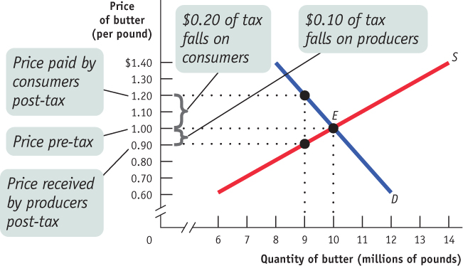
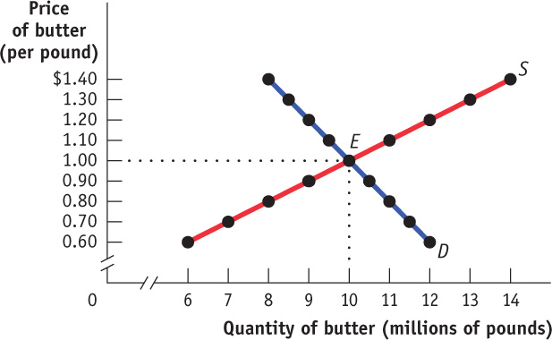
1. Consider the market for butter, shown in the accompanying figure. The government imposes an excise tax of $0.30 per pound of butter. What is the price paid by consumers post-tax? What is the price received by producers post-tax? What is the quantity of butter sold? How is the incidence of the tax allocated between consumers and producers? Show this on the figure.

2. The accompanying table shows five consumers’ willingness to pay for one can of diet soda each as well as five producers’ costs of selling one can of diet soda each. Each consumer buys at most one can of soda; each producer sells at most one can of soda. The government asks your advice about the effects of an excise tax of $0.40 per can of diet soda. Assume that there are no administrative costs from the tax.

Consumer	Willingness to Pay	Producer	Cost
Ana	$0.70	Zhang	$0.10
Bernice	0.60	Yves	0.20
Chizuko	0.50	Xavier	0.30
Dagmar	0.40	Walter	0.40
Ella	0.30	Vern	0.50

• a. Without the excise tax, what is the equilibrium price and the equilibrium quantity of soda?

• b. The excise tax raises the price paid by consumers post-tax to $0.60 and lowers the price received by producers post-tax to $0.20. With the excise tax, what is the quantity of soda sold?

• c. Without the excise tax, how much individual consumer surplus does each of the consumers gain? How much individual consumer surplus does each consumer gain with the tax? How much total consumer surplus is lost as a result of the tax?

• d. Without the excise tax, how much individual producer surplus does each of the producers gain? How much individual producer surplus does each producer gain with the tax? How much total producer surplus is lost as a result of the tax?

• e. How much government revenue does the excise tax create?

• f. What is the deadweight loss from the imposition of this excise tax?

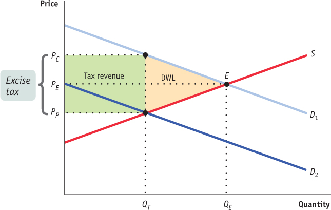
Draw a correctly labeled graph of a competitive market in equilibrium. Use your graph to illustrate the effect of an excise tax imposed on consumers. Indicate each of the following on your graph:

• a. the equilibrium price and quantity without the tax, labeled P_E and Q_E
• b. the quantity sold in the market post-tax, labeled Q_T
• c. the price paid by consumers post-tax, labeled P_C
• d. the price received by producers post-tax, labeled P_P
• e. the tax revenue generated by the tax, labeled “Tax revenue”
• f. the deadweight loss resulting from the tax, labeled “DWL”
• g. the wedge created by the tax between P_C and P_P, labeled “Excise tax”